This chapter was written by Lean Fang, Seth Zoppelt, and Zilong Li and reviewed by Ping He.
Learning Objectives:
After reading this chapter, you should be able to:
-
Setup aerodynamic optimizations for subsonic and transonic conditions
-
Setup multi-point optimizations to consider multiple flow conditions
-
Setup multi-case optimizations where each case runs in a separate folder
Subsonic optimization
The following is the overview of an aerodynamic shape optimization case for the NACA0012 airfoil in subsonic conditions.
Case: Airfoil aerodynamic optimization
Geometry: NACA0012
Objective function: Drag coefficient (CD)
Lift coefficient (CL): 0.5
Design variables: 20 free-form deformation (FFD) points moving in the y direction, one angle of attack
Constraints: Symmetry, volume, thickness, and lift constraints (total number: 34)
Mach number: 0.294 (100 m/s)
Reynolds number: 6.667 million
Mesh cells: ~4,500
Solver: DARhoSimpleFoam
The “runScript.py” is similar to the one used in the NACA0012 incompressible case with the following exceptions:
- In the global parameters, we provide additional variable such as “T0” (far field temperature) and “rho0” (a reference density to normalize CD and CL). In addition, we provide the absolute value of pressure “p”, instead of the relative value use in the low speed case.
# =============================================================================
# Input Parameters
# =============================================================================
U0 = 100.0
p0 = 101325.0
T0 = 300.0
nuTilda0 = 4.5e-5
CL_target = 0.5
aoa0 = 4.0
A0 = 0.1
# rho is used for normalizing CD and CL
rho0 = p0 / T0 / 287
-
In “primalBC”, we need to set boundary condition for temperature “T0”.
-
We use “DARhoSimpleFoam”, which is an OpenFOAM built-in compressible flow solver suitable for subsonic conditions. Accordingly, we set “flowCondition” to “Compressible”.
# Input parameters for DAFoam
daOptions = {
    "designSurfaces": ["wing"],
    "solverName": "DARhoSimpleFoam",
    "primalMinResTol": 1.0e-8,
    "primalBC": {
        "U0": {"variable": "U", "patches": ["inout"], "value": [U0, 0.0, 0.0]},
        "p0": {"variable": "p", "patches": ["inout"], "value": [p0]},
        "T0": {"variable": "T", "patches": ["inout"], "value": [T0]},
        "nuTilda0": {"variable": "nuTilda", "patches": ["inout"], "value": [nuTilda0]},
        "useWallFunction": True,
    },
    "function": {
        "CD": {
            "type": "force",
            "source": "patchToFace",
            "patches": ["wing"],
            "directionMode": "parallelToFlow",
            "patchVelocityInputName": "patchV",
            "scale": 1.0 / (0.5 * U0 * U0 * A0 * rho0),
        },
        "CL": {
            "type": "force",
            "source": "patchToFace",
            "patches": ["wing"],
            "directionMode": "normalToFlow",
            "patchVelocityInputName": "patchV",
            "scale": 1.0 / (0.5 * U0 * U0 * A0 * rho0),
        },
    },
    "adjEqnOption": {"gmresRelTol": 1.0e-6, "pcFillLevel": 1, "jacMatReOrdering": "rcm"},
    "normalizeStates": {
        "U": U0,
        "p": p0,
        "T": T0,
        "nuTilda": nuTilda0 * 10.0,
        "phi": 1.0,
    },
    "inputInfo": {
        "aero_vol_coords": {"type": "volCoord", "components": ["solver", "function"]},
        "patchV": {
            "type": "patchVelocity",
            "patches": ["inout"],
            "flowAxis": "x",
            "normalAxis": "y",
            "components": ["solver", "function"],
        },
    },
}
Some files under 0.orig are also different from the incompressible case due to the compressible solver “DARhoSimpleFoam”.
-
DARhoSimpleFoam for subsonic flow has an extra field variable called “alphat”.
-
DARhoSimpleFoam’s pressure p has the dimension [1 -1 -2 0 0 0 0], meaning kg / (m s2), while the pressure p for the incompressible DASimpleFoam has the dimension [0 2 -2 0 0 0 0], meaning m2 / s2. The pressure for the incompressible DASimpleFoam is relative, and we ues zero as the reference value; while the pressure for the compressible DARhoSimpleFoam is absolute and always non-zero.
Similarly, some files under the constant folder are also different.
- DARhoSimpleFoam uses “thermophysicalProperties” while DASimpleFoam uses “transportProperties”.
Note: the fvSchemes and fvSolution files under system are also different for a subsonic case using DARhoSimpleFoam. When setting up your own subsonic case, please use the fvSchemes and fvSolution files linked here as the template.
Transonic optimization
The following is the overview of an aerodynamic shape optimization case for the NACA0012 airfoil in transonic conditions.
Case: Airfoil aerodynamic optimization
Geometry: NACA0012
Objective function: Drag coefficient (CD)
Lift coefficient (CL): 0.5
Design variables: 20 free-form deformation (FFD) points moving in the y direction, one angle of attack
Constraints: Symmetry, volume, thickness, and lift constraints (total number: 34)
Mach number: 0.7 (238 m/s)
Reynolds number: 15.9 million
Mesh cells: ~4,500
Solver: DARhoSimpleCFoam
The “runScript.py” is similar to the one used in the NACA0012 subsonic case mentioned above with the following exceptions:
-
We use “DARhoSimpleCFoam”, which is an OpenFOAM built-in compressible flow solver with the “SIMPLEC” algorithm that is suitable for transonic conditions.
-
The far field velocity is 238 m/s with Mach number of 0.7.
-
We use special treatment for the preconditioner matrix to improve the convergence of adjoint linear equation by setting “transonicPCOption”: 1. This option is only needed for transonic conditions.
Note: the fvSchemes and fvSolution files under system are also different for a transonic case using DARhoSimpleCFoam. When setting up your own transonic case, please use the fvSchemes and fvSolution files linked here as the template.
Multi-point optimization
With multipoint optimization, we make some subtle changes to the runScript (see /tutorials/NACA0012_Airfoil/Incompressible for the original runScript). When defining the global parameters, we have now
# we have two flight conditions
weights = [0.5, 0.5]
U0 = [10.0, 5.0]
p0 = 0.0
nuTilda0 = 4.5e-5
aoa0 = [5.0, 4.0]
A0 = 0.1
# rho is used for normalizing CD and CL
rho0 = 1.0
scalings = [1.0 / (0.5 * A0 * rho0 * U0[0] * U0[0]), 1.0 / (0.5 * A0 * rho0 * U0[1] * U0[1])]
lift_target = [0.5 / scalings[0], 0.4 / scalings[1]]
Now, we set weights to each scenario (here, they are weighted the same). Since we have two scenarios, there are two sets of initial conditions and two targets for $C_L$. Most of the runScript is the same as the incompressible, low-speed NACA0012 case, but we make some changes in the Top class. In the setup, we make the following changes:
# add a scenario (flow condition) for optimization, we pass the builder
# to the scenario to actually run the flow and adjoint
self.mphys_add_scenario("scenario1", ScenarioAerodynamic(aero_builder=dafoam_builder))
self.mphys_add_scenario("scenario2", ScenarioAerodynamic(aero_builder=dafoam_builder))

# need to manually connect the x_aero0 between the mesh and geometry components
# here x_aero0 means the surface coordinates of structurally undeformed mesh
self.connect("mesh.x_aero0", "geometry.x_aero_in")
# need to manually connect the x_aero0 between the geometry component and the cruise
# scenario group
self.connect("geometry.x_aero0", "scenario1.x_aero")
self.connect("geometry.x_aero0", "scenario2.x_aero")

# add an exec comp to average two drags, the weights are 0.5 and 0.5
self.add_subsystem(
    "obj",
        om.ExecComp(
            "val=w1*drag1+w2*drag2",
            w1={"val": weights[0] * scalings[0], "constant": True},
            w2={"val": weights[1] * scalings[1], "constant": True},
        ),
    )
Most importantly, we add two scenarios using mphys_add_scenario. Note that we use the same dafoam_builder. We also connect the geometry to each scenario, which implies that we use the same geometry and same mesh to run each scenario. We then create the objective function as a weighted average of the drags from each scenario. At the end of the configuration setup in def(configure), we make the following changes:
# add the design variables to the dvs component's output
self.dvs.add_output("shape", val=np.array([0] * len(shapes)))
# NOTE: we have two separated aoa variables for the two flight conditions
self.dvs.add_output("patchV1", val=np.array([U0[0], aoa0[0]]))
self.dvs.add_output("patchV2", val=np.array([U0[1], aoa0[1]]))
# manually connect the dvs output to the geometry and cruise
self.connect("patchV1", "scenario1.patchV")
self.connect("patchV2", "scenario2.patchV")
self.connect("shape", "geometry.shape")

# define the design variables to the top level
self.add_design_var("shape", lower=-1.0, upper=1.0, scaler=10.0)
self.add_design_var("patchV1", lower=[U0[0], 0.0], upper=[U0[0], 10.0], scaler=0.1)
self.add_design_var("patchV2", lower=[U0[1], 0.0], upper=[U0[1], 10.0], scaler=0.1)

# add objective and constraints to the top level
# we have two separated lift constraints for for the two flight conditions
self.add_constraint("scenario1.aero_post.lift", equals=lift_target[0], scaler=1.0)
self.add_constraint("scenario2.aero_post.lift", equals=lift_target[1], scaler=1.0)
self.add_constraint("geometry.thickcon", lower=0.5, upper=3.0, scaler=1.0)
self.add_constraint("geometry.volcon", lower=1.0, scaler=1.0)
self.add_constraint("geometry.rcon", lower=0.8, scaler=1.0)

# here we use the obj.val defined above as the obj func.
self.add_objective("obj.val", scaler=1.0)
self.connect("scenario1.aero_post.drag", "obj.drag1")
self.connect("scenario2.aero_post.drag", "obj.drag2")
The main changes above that we make are adding two patches in the dvs, patchV1 and patchV2. Note that the initial values that we assign for U0 and aoa0 are indexed to align with their respective scenario and patch. Then, we connect the patchV from each scenario to the respective patchV1 and patchV2. Below, we then add design our design variables, again noting that there is now a design variable for each patch, labeled as such. Then , we need to add our constraints. Looking at the lift constraint, we add one for each scenario, and assign the constraint from the list, list_target. Finally, we add our objective function that was defined above. We add connections for each scenario once again, shown above. Finally, we need to make some changes for the optimization task:
if args.task == "run_driver":
    # solve CL
    optFuncs.findFeasibleDesign(
        ["scenario1.aero_post.lift", "scenario2.aero_post.lift"],
        ["patchV1", "patchV2"],
        designVarsComp=[1, 1],
        targets=lift_target,
    )
    # run the optimization
    prob.run_driver()
The change we make is in the optFuncs.findFeasibleDesign. We have to add the $C_L$ target from each scenario, aligning the lift, patchV’s, and designVarsComp from each case (note that lift_target is a 2-element array).
After running the optimization, we can see the N2 diagram below.
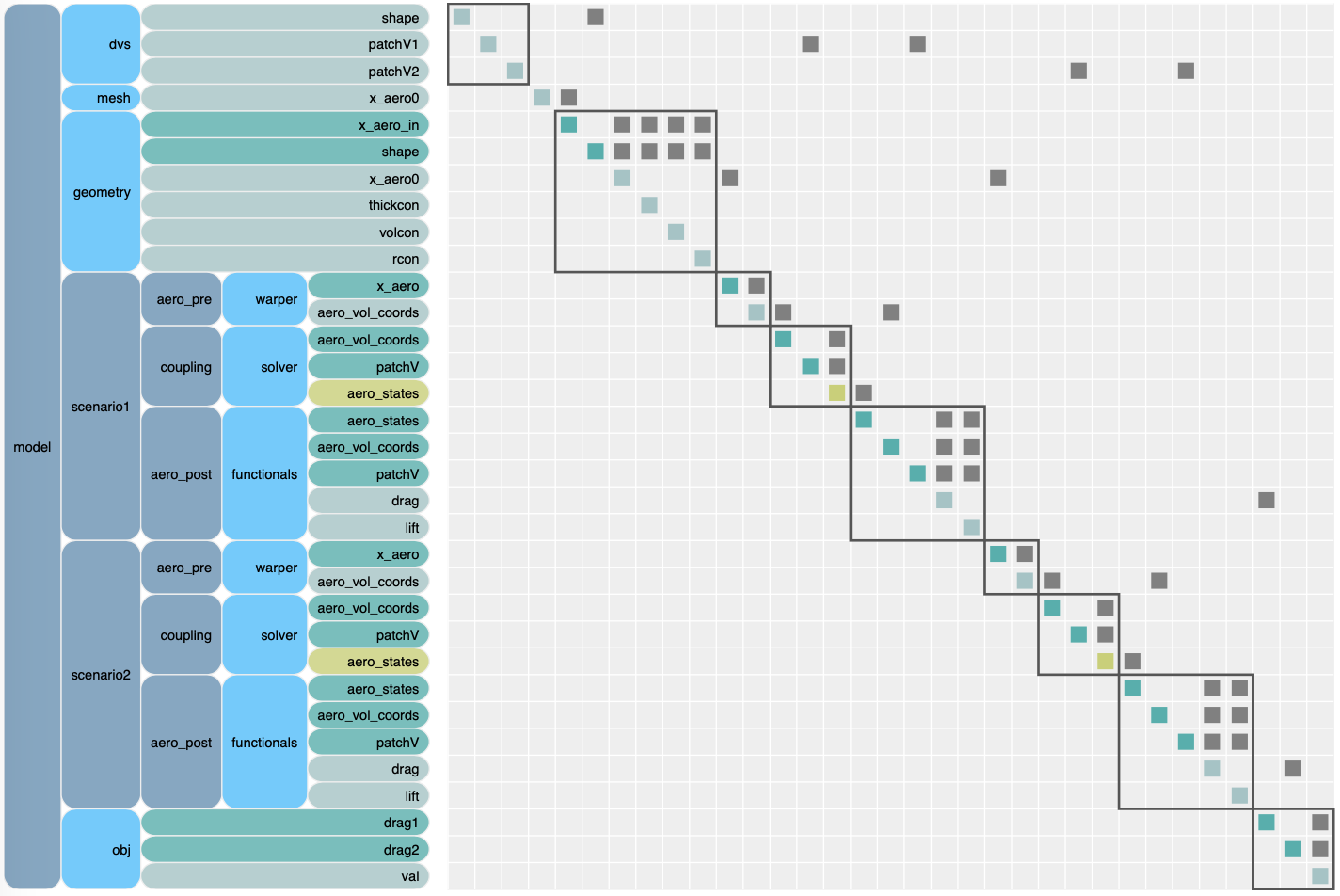
Examining the N2 diagram, we observe that there is only one geometry, and the x_aero0 from the geometry is linked to x_aero0 in both scenarios, which both are displayed on the N2 diagram.
Overall, multipoint optimization is used when relatively simple parameters are to be changed to run multiple cases at once, but the overall structure of the optimization setup remains the same. In this case, the only changes between cases were the initial velocity, angle of attack, and the $C_L$ target. The geometry, solver, turbulence model, etc. all remain the same, so multipoint is the ideal setup to use (rather than multicase, shown below). Place holder text, don’t change!
Multi-case optimization
The following is a multi-case aerodynamic shape optimization problem for the NACA0012 airfoil. This tutorial will show you how to use one runScript.py to run multiple cases within one folder. Go to the directory: /tutorials-master/NACA0012_Airfoil/multicase, and we will see two subdirectories, SA and SST, which are the two cases we are going to run.
The “runScript.py” for the multi-case is mostly like the NACA0012 incompressible case, except that we need to provide the parameters required for the SST model, such as “k0” and “omega0”.
# =============================================================================
# Input Parameters
# =============================================================================
U0 = 10.0
p0 = 0.0
nuTilda0 = 4.5e-5
k0 = 0.015
omega0 = 100.0
CL_target = 0.5
aoa0 = 5.0
A0 = 0.1
rho0 = 1.0
Just like the SA model, we also need to provide the daOptions for the SST model. For descriptions of the parameters, one can refer to the NACA0012 incompressible case.
daOptionsSST = {
    "designSurfaces": ["wing"],
    "solverName": "DASimpleFoam",
    "primalMinResTol": 1.0e-8,
    "primalBC": {
        "U0": {"variable": "U", "patches": ["inout"], "value": [U0, 0.0, 0.0]},
        "p0": {"variable": "p", "patches": ["inout"], "value": [p0]},
        "k0": {"variable": "k", "patches": ["inout"], "value": [k0]},
        "omega0": {"variable": "omega", "patches": ["inout"], "value": [omega0]},
        "useWallFunction": True,
    },
    "function": {
        "CD": {
            "type": "force",
            "source": "patchToFace",
            "patches": ["wing"],
            "directionMode": "parallelToFlow",
            "patchVelocityInputName": "patchV",
            "scale": 1.0 / (0.5 * U0 * U0 * A0 * rho0),
        },
        "CL": {
            "type": "force",
            "source": "patchToFace",
            "patches": ["wing"],
            "directionMode": "normalToFlow",
            "patchVelocityInputName": "patchV",
            "scale": 1.0 / (0.5 * U0 * U0 * A0 * rho0),
        },
    },
    "adjEqnOption": {"gmresRelTol": 1.0e-6, "pcFillLevel": 1, "jacMatReOrdering": "rcm"},
    "normalizeStates": {
        "U": U0,
        "p": U0 * U0 / 2.0,
        "k": k0,
        "omega": omega0,
        "phi": 1.0,
    },
    "inputInfo": {
        "aero_vol_coords": {"type": "volCoord", "components": ["solver", "function"]},
        "patchV": {
            "type": "patchVelocity",
            "patches": ["inout"],
            "flowAxis": "x",
            "normalAxis": "y",
            "components": ["solver", "function"],
        },
    },
}
Then, we need to create the builder to initialize the DASolvers for both cases in the setup(self) function, and the most important change we make here is that we need to use the “run_directory” entry, we need to specify one is for the SA model and the other is for the SST model (for new cases, such as when running a multi-case optimization problem for both subsonic and transonic cases, we may need to make corresponding changes to the “run_directory”), and after that, we can add the mesh, geometry, and scenario components for both cases. The primary benefit of a multi-case run is that within one folder, we can run the optimization across different cases. Note that within that folder, the SA subfolder and the SST subfolder should have their own “0”, “constant”, and “system” directories, etc.
def setup(self):
    # create the builder to initialize the DASolvers for both cases (they share the same mesh option)
    dafoam_builder_sa = DAFoamBuilder(daOptionsSA, meshOptions, scenario="aerodynamic", run_directory="SA")
    dafoam_builder_sa.initialize(self.comm)
    dafoam_builder_sst = DAFoamBuilder(daOptionsSST, meshOptions, scenario="aerodynamic", run_directory="SST")
    dafoam_builder_sst.initialize(self.comm)

    # add the mesh component
    self.add_subsystem("mesh_sa", dafoam_builder_sa.get_mesh_coordinate_subsystem())
    self.add_subsystem("mesh_sst", dafoam_builder_sst.get_mesh_coordinate_subsystem())

    # add the geometry component (FFD)
    self.add_subsystem("geometry_sa", OM_DVGEOCOMP(file="SA/FFD/wingFFD.xyz", type="ffd"))
    self.add_subsystem("geometry_sst", OM_DVGEOCOMP(file="SST/FFD/wingFFD.xyz", type="ffd"))

    # add a scenario (flow condition) for optimization, we pass the builder
    # to the scenario to actually run the flow and adjoint
    self.mphys_add_scenario("scenario_sa", ScenarioAerodynamic(aero_builder=dafoam_builder_sa))
    self.mphys_add_scenario("scenario_sst", ScenarioAerodynamic(aero_builder=dafoam_builder_sst))

    # need to manually connect the x_aero0 between the mesh and geometry components
    # here x_aero0 means the surface coordinates of structurally undeformed mesh
    self.connect("mesh_sa.x_aero0", "geometry_sa.x_aero_in")
    self.connect("geometry_sa.x_aero0", "scenario_sa.x_aero")

    self.connect("mesh_sst.x_aero0", "geometry_sst.x_aero_in")
    self.connect("geometry_sst.x_aero0", "scenario_sst.x_aero")
In the configure(self) function, we also need to provide the corresponding parameters for both the SA and SST models. For descriptions of the parameters, one can refer to the NACA0012 incompressible case.
def configure(self):
    # get the surface coordinates from the mesh component
    points_sa = self.mesh_sa.mphys_get_surface_mesh()
    points_sst = self.mesh_sst.mphys_get_surface_mesh()

    # add pointset to the geometry component
    self.geometry_sa.nom_add_discipline_coords("aero", points_sa)
    self.geometry_sst.nom_add_discipline_coords("aero", points_sst)

    # set the triangular points to the geometry component for geometric constraints
    tri_points_sa = self.mesh_sa.mphys_get_triangulated_surface()
    self.geometry_sa.nom_setConstraintSurface(tri_points_sa)
    tri_points_sst = self.mesh_sst.mphys_get_triangulated_surface()
    self.geometry_sst.nom_setConstraintSurface(tri_points_sst)

    self.geometry_sa.nom_addShapeFunctionDV(dvName="shape", shapes=shapes)
    self.geometry_sst.nom_addShapeFunctionDV(dvName="shape", shapes=shapes)

    # add the design variables to the dvs component's output
    self.dvs.add_output("shape", val=np.array([0] * len(shapes)))
    self.dvs.add_output("patchV_sa", val=np.array([U0, aoa0]))
    self.dvs.add_output("patchV_sst", val=np.array([U0, aoa0]))

    # manually connect the dvs output to the geometry and cruise
    # sa and sst cases share the same shape
    self.connect("patchV_sa", "scenario_sa.patchV")
    self.connect("shape", "geometry_sa.shape")
    self.connect("patchV_sst", "scenario_sst.patchV")
    self.connect("shape", "geometry_sst.shape")

    # define the design variables to the top level
    self.add_design_var("shape", lower=-1.0, upper=1.0, scaler=10.0)
    self.add_design_var("patchV_sa", lower=[U0, 0.0], upper=[U0, 10.0], scaler=0.1)
    self.add_design_var("patchV_sst", lower=[U0, 0.0], upper=[U0, 10.0], scaler=0.1)

    # add objective and constraints to the top level
    self.connect("scenario_sa.aero_post.CD", "obj.cd_sa")
    self.connect("scenario_sst.aero_post.CD", "obj.cd_sst")
    self.add_constraint("scenario_sa.aero_post.CL", equals=CL_target, scaler=1.0)
    self.add_constraint("scenario_sst.aero_post.CL", equals=CL_target, scaler=1.0)
In this case, we optimize the case using both SA and SST models, and the objective function is the averaged drag between SA and SST. So we need to add an “obj” subsystem in the setup(self) function, and set the “value=(cd_sa+cd_sst)/2”). Then, in the configure(self) function, we can use the “obj.value” as the entry for the objective function.
def setup(self):
    self.add_subsystem("obj", om.ExecComp("value=(cd_sa+cd_sst)/2"))
def configure(self):
    self.add_objective("obj.value", scaler=1.0)
The N2 diagram will output as .html, which can be opened within a web browser. This is an interactive diagram that can help you visualize your connections within your optimization framework.
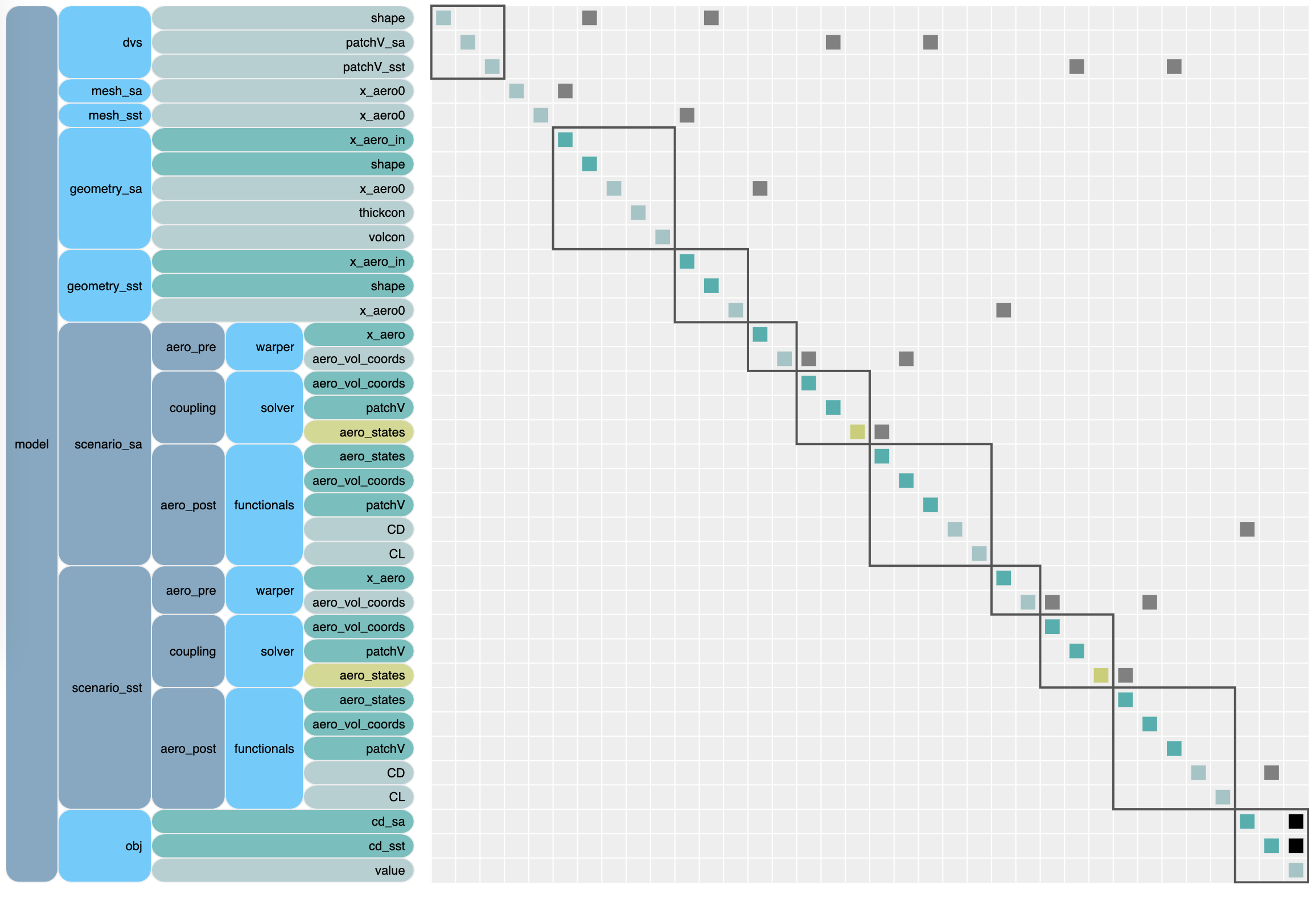
Fig. 1. The N2 diagram for the multi-case optimization.
Questions
1. Transonic
Set up a new transonic airfoil case:
- Use NREL S809 airfoil as the baseline design
- Use 10 FFD points along the chord direction
- Use a finer structured mesh generated by pyHyp with 50,000 to 100,000 cells
- The average y+ value should be between 0.5 and 3
- The Reynolds number is 5 × 10⁶
- The Mach number is 0.75
- The target CL is 0.6
After this new airfoil optimization case converges,
- What is the optimized CD, and how much reduction in CD have you achieved?
- What is the optimized airfoil shape?
2. Multi-point
There is another scenario that will be added to the multi-point case up above. This scenario will have the following flight conditions:
\[\begin{aligned} U_0 = 15.0 \\ \alpha = 3.0 \\ \text{weight} = 0.3 \end{aligned}\]Note that the weights for the previous flight conditions will now be $\text{weight}=0.35$ each.
a) Update the runScript.py file inside tutorials/NACA0012_Airfoil/multipoint to add this third case that is described up above. Provide your updated scaling, lift target, and objective function.
b) Provided the updated $N^2$ diagram.
c) Provided the results of the optimization.
3. Multi-case Set up a new multi-case (low-speed and transonic cases) optimization:
- Use the NACA0012 as the baseline design (you can reuse the information in the existing multicase tutorial, such as mesh, FFD points, profiles, etc.)
- The low-speed case Mach number is 0.3
- The transonic case Mach number is 0.75
- The target CL for the low-speed case is 0.5
- The target CL for the transonic case is 0.6
After this multi-case optimization is done:
- Provide the N2 diagram
- Report the optimized CD, and compute the CD reduction
- Show the optimized airfoil shape.
Place holder text, don’t change!