The following is an aerodynamic shape optimization case for the Rotor37 axial compressor rotor.
Case: Axial compressor aerodynamic optimization at transonic conditions
Geometry: Rotor37
Objective function: Torque
Design variables: 50 FFD points moving in the y and z directions
Constraints: Constant mass flow rate and total pressure ratio
Rotation speed: 1800 rad/s
Mesh cells: 40 K
Adjoint solver: DATurboFoam
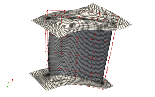
Fig. 1. Mesh and FFD points for the Rotor37 case
To run this case, first download tutorials and untar it. Then go to tutorials-main/Rotor37_Compressor and run the “preProcessing.sh” script to generate the mesh:
./preProcessing.sh
Then, use the following command to run the optimization with 4 CPU cores:
mpirun -np 4 python runScript.py 2>&1 | tee logOpt.txt
Post Procesing:
Use the following command to load the OpenFOAM environment:
of1812
Next, run the following command:
reconstructPar
This will generate new folders and allow the deletion of all of the processor folders. This makes the entire directory a bit smaller and allow for easier processing.
Open the paraview.foam file in the ParaView application. Check the boxes next to blade and hub and uncheck the box next to mesh. After hitting apply, the blade will appear on the viewer. This will show the pressure gradient by default. There is a play button at the top of the window that will show all iterations through each timestep of the optimization. The original blade should look like figure 2 and figure 3 as the top and bottom, respectively.
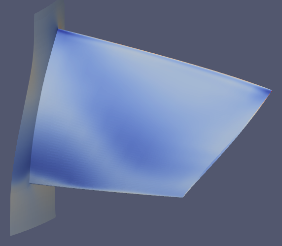
Fig. 2. Pressure gradient on the top of the original blade
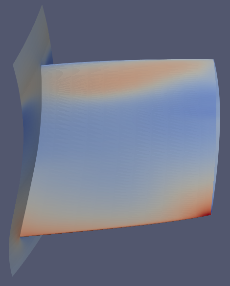
Fig. 3. Pressure gradient on the bottom of the orignal blade
After optimizaiton, the pressure gradients should look as follows:
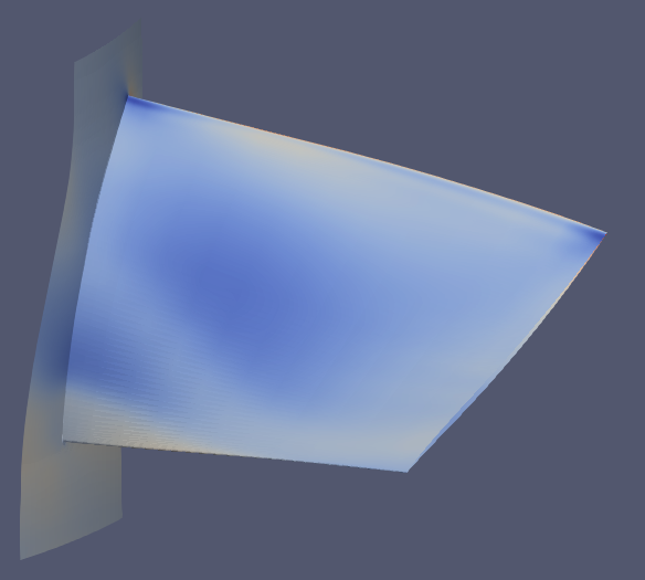
Fig. 4. Pressure gradient on the top of the optimized blade
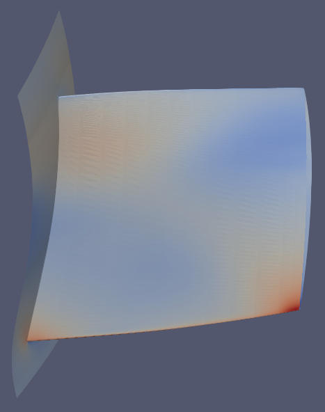
Fig. 5. Pressure gradient on the bottom of the optimized blade
After this, the blade can be sliced using a cylindrical slice. The slices allow the profile of the blade to be viewed. Figures 6 and 7 show a comparison of the original blade vs the optimized blade at the root and at the tip.
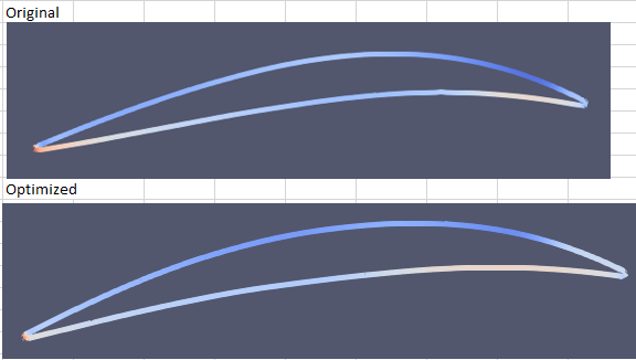
Fig. 6. The original airfoil and the optimized airfoil at the root
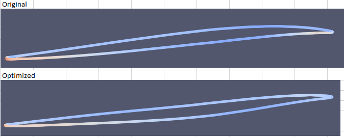
Fig. 7. The original airofil and the optimized airfoil at the tip
On each slice, use the “Plot on sorted lines” filter to achieve a graph of the pressure distribution accross the airfoil. Figures 8 and 9 show overlayed plots of the orignal shape and the optimized shape at the root and at the tip.
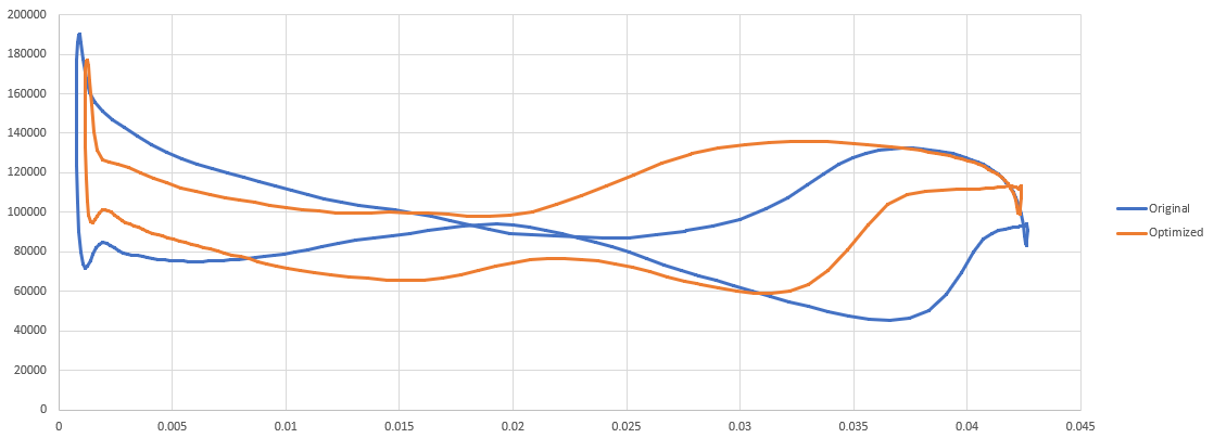
Fig. 8. Overlayed plot of pressure distribution at the root
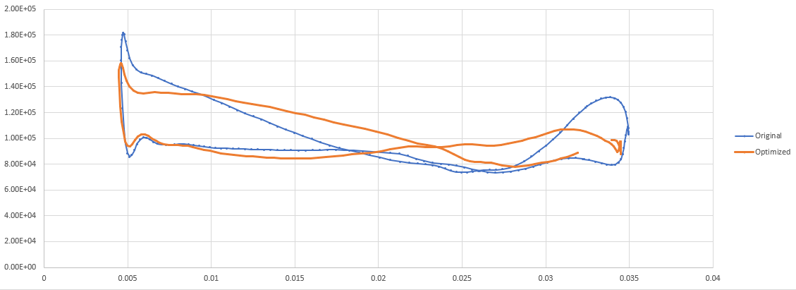
Fig. 9. Overlayed plot of pressure distribution at the tip
To see the Mach gradiant, check the box next to mesh and uncheck the blade and hub. The slice will update to show the mesh. This will need to be coppied 4 or 5 more times, with each slice being translated up by 10°. A calculator needs to be put onto each slice to calculate the Mach number. The Mach number can then be selected to view instead of the pressure. Figures 10 and 11 show the Mach gradients for both the original and optimized cases at the root and at the tip.
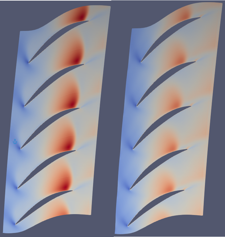
Fig. 10. Mach gradient at root, left is original and right is optimized
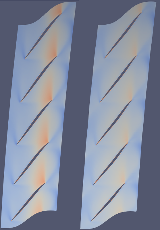
Fig. 11. Mach gradient at tip, left is orignal and right is optimized