The following is an aerodynamic shape optimization case for the DPW4 aircraft (wing-body-tail configuration) at transonic conditions.
Case: Aircraft aerodynamic optimization
Geometry: CRM wing, body, and tail
Objective function: Drag coefficient
Design variables: 216 FFD points moving in the z direction, 9 wing twists, one tail rotation, one angle of attack
Constraints: Volume, thickness, LE/TE, and lift constraints (total number: 771)
Mach number: 0.85
Reynolds number: 5 million
Mesh cells: 860 K
Solver: DARhoSimpleCFoam

Fig. 1. Mesh and FFD points for the DPW4 wing-body-tail configuration
To run this case, first download tutorials and untar it. Then go to tutorials-main/DPW4_Aircraft and run the “preProcessing.sh” script to generate the mesh:
./preProcessing.sh
We recommend running this case on an HPC system with 100 CPU cores:
mpirun -np 100 python runScript.py 2>&1 | tee logOpt.txt
To complete the post-processing for this case, first load the OpenFOAM environment. Next, run the following command:
reconstructPar
This will generate new folders and allow the deletion of all the processor folders. This makes the entire directory smaller and allows for easier processing.
After the deletion is complete, download and extract the entire directory to an accessible location.
Then, open Paraview and open the “paraview.foam” file. First, make sure that the case type selected is “reconstructed”. Then select all mesh regions except “internalMesh” and “patch/inout”. Finally, check the box that says “Camera Parallel Projection”. Click “Apply” to view a colored pressure gradient on the DPW4 Aircraft. For more details related to post processing, refer to the post-processing page in Get Started.
This optimization was completed with a goal of minimizing the CD while maintaining the CL. This case ran for 63 major optimization iterations, completed over 51 hours with 108 cores on the Nova HPC. According to “opt_SNOPT_summary.txt”, the original CD was 0.041765362 and the optimized CD was 0.038138414, which is an 8.7% drag reduction. This reduction is significant and comes as a direct result of shaping improvements.
Fig. 2. Complete optimization animation with Cp gradient, iterations, drag reduction, lift coefficient, and moment coefficient visible.
Since the body, wings, and tail are mirrored over the central axis, a view of one half of the airplane provides the simplest look at the changes to the shape over time. In Figures 3, 4, and 5 below, we can see several views of the original versus final shapes of the wing, body, and tail.
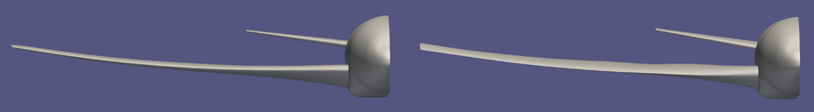
Fig. 3. Front view of baseline shape (left) and optimized shape (right)
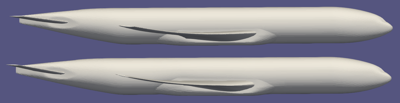
Fig. 4. Side view of baseline shape (top) and optimized shape (bottom)
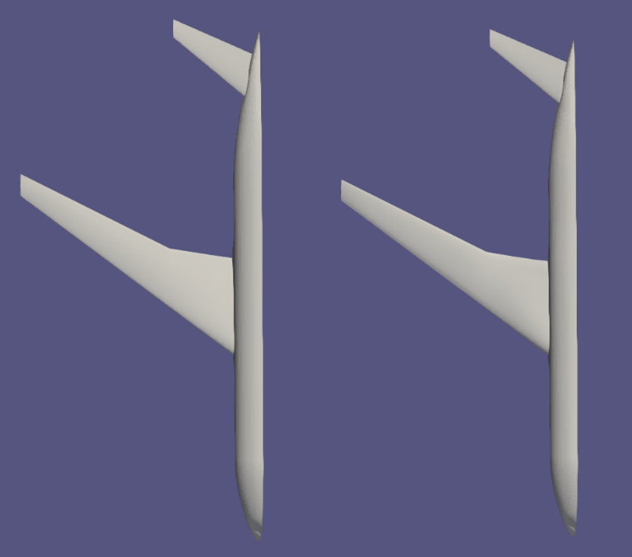
Fig. 5. Top view of baseline shape (left) and optimized shape (right)
As evident in the figures provided, many of the improvements to the CD are a direct result of an improved angle of the wing and tail. While there are certainly changes to the thickness of the airfoils, the outline of the wing as seen from above is barely affected. Rather, as seen in the side view, the main wing and front portion of the tail seem to have been rotated slightly downward.
In addition to these visuals indicating the changes to the shape of the aircraft, an analysis of variables affected by the optimization can help identify the strongest points of improvement. A primary variable to be examined is pressure, where the location and overall areas of high and low pressure contribute directly to CL and CD.
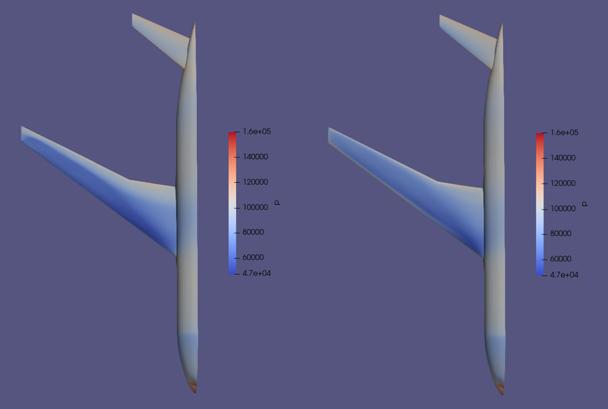
Fig. 6. Top-down view of baseline (left) and optimized pressure field (right)
Figure 6 provides a clear view of the change in pressure distribution. In the baseline shape, shown on the left, a large area of low pressure is present near the leading edge of the wing, tapering off near the trailing edge and increasing in pressure near both the outer and inner sections of the wing. In the optimized shape, we can see the pressure gradient is much more evenly distributed, with the areas of low pressure shifting backward and inward, demonstrating a cleaner airflow over the wing.
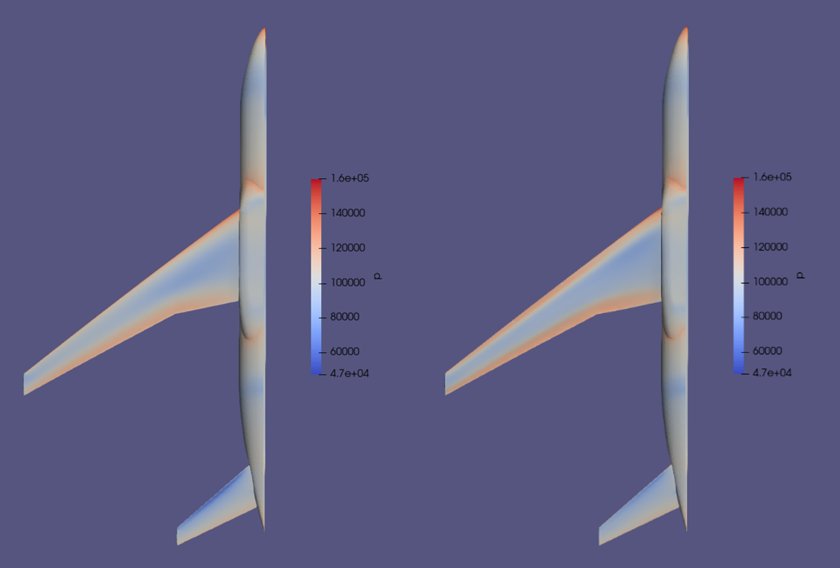
Fig. 7. Bottom-up view of baseline (left) and optimized pressure field (right)
Figure 7 has a less pronounced change in the pressure gradient than Figure 6, but the differences are relevant. In the baseline view, the trailing edge of the wing has a distinctly higher pressure, which fades near both the inner and outer edges of the wing. Additionally, the low-pressure area in the center of the wing takes up a significant amount of the surface area, with the lowest pressure center spreading out over the inner wing area. Besides the wing itself, changes in the tail are more visible in this figure, too. The baseline tail has a strong low-pressure area spanning almost the entire leading edge, which is not optimal.
The optimized pressure gradient for both the wing and tail improves many of these issues noted in the baseline shape. The leading edge of the wing now has a slightly more pronounced high-pressure span, which does not immediately fade. The large low-pressure area noted in the baseline has spread out, distributing more evenly and increasing in overall pressure. The trailing edge also now reaches fully from the wing tip to the inner wing, avoiding the gradient cutoff noted in the baseline. The tail additionally shows improvement, with the strong low-pressure area increasing significantly in pressure.
One constraint to note is that all the analyzed results for pressure are relative to the very high pressure applied on the front nose of the main aircraft body, making the differences in wing pressure less pronounced. Still, the improvements noted above are visible, which is a testament to the overall improvement of this optimization.
Also note an analysis of the pressure helps give a general idea of the improvements in CD, but visualizing the velocity streamlines allows for a much more direct view of the improved airflow.
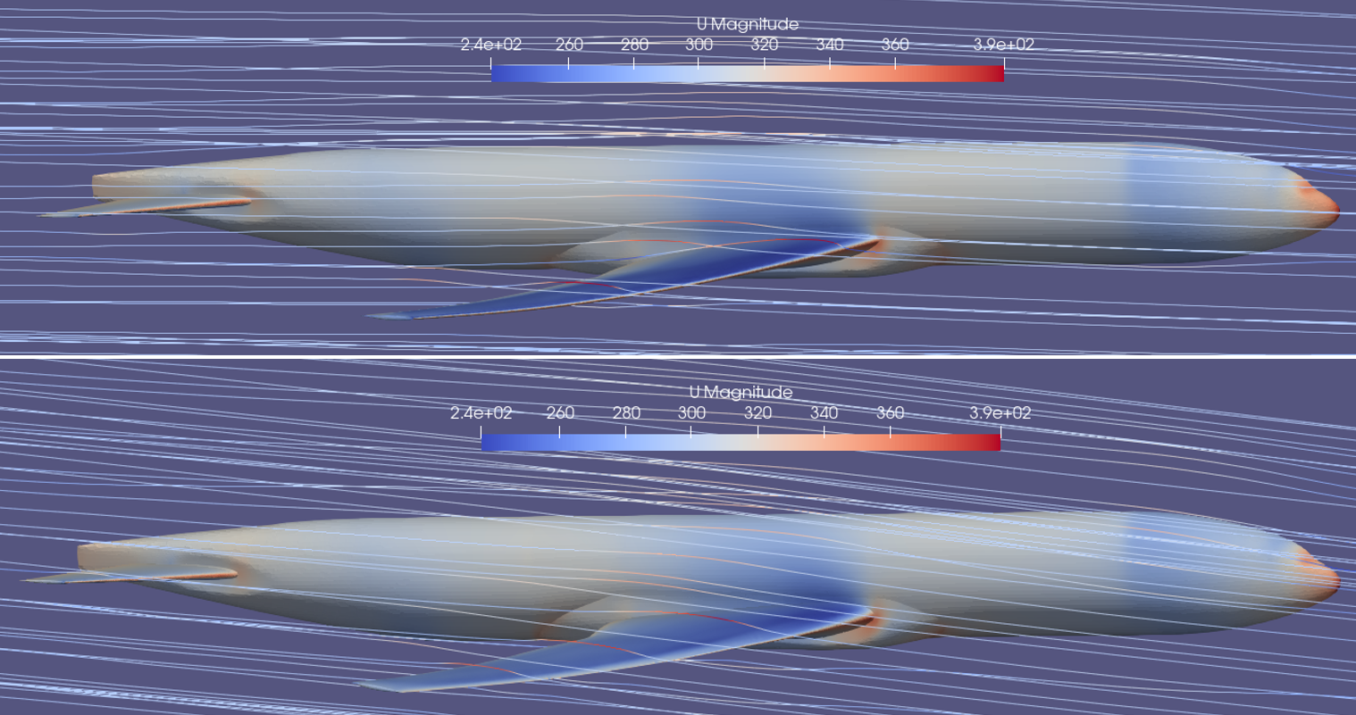
Fig. 8. Side view of baseline (top) and optimized streamline velocities (bottom)
The primary differences between the baseline and optimized streamlines become clearer when compared to an “optimal” airflow. Ideally, airflow over the top of the wing should be of a higher velocity than that of the bottom of the wing, creating the low-pressure area seen earlier. In the baseline view, the higher velocity is present, but is visible only near the leading edge of the wing. This is the reason the low-pressure area is much more concentrated near the leading edge of the wing in Figure 6, resulting in an increased CD. However, in the optimized view, we can see the higher velocity streamlines continue over much more of the wing area, and are less pronounced near the leading edge. This contributes directly to the more evenly distributed pressure gradient, additionally improving the CD.
Finally, a general overview of the improvements is easily created by comparing the CD and overall major iterations of the optimization.
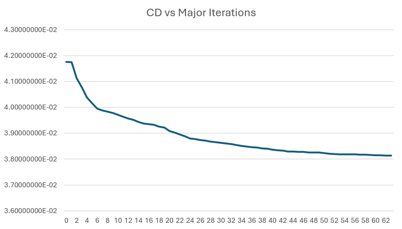
Fig. 9. Line plot of CD versus Major Iterations of the optimization (0-63)
The plot in Figure 9 begins at major iteration 0, indicating the first CD value of 4.1765362E-02 by the short horizontal starting line. This is followed by a sharp decrease in the following major iterations, as is typical with these optimizations. As the tenth major iteration is approached (CD of 3.97E-02), the steep slope evens out into what almost resembles a linear downward path, steadily decreasing until nearly iteration 45 (CD of 3.83E-02). At that point, the curve begins to flatten, representing the final decrease from 3.83E-02 to ~3.81E-02.