Steady flow
The following is a data-assimilation optimization case where we try to find the velocity magnitude, angle of attack, and airfoil geometry based on pressure data on the NACA0012 airfoil.
Case: Data assimilation optimization (steady-state)
Geometry: NACA0012
Objective function: Pressure prediction errors on the airfoil
Design variables: Velocity magnitude, angle of attack at the far field, and the shape of the airfoil
Constraints: None
Reynolds number: 0.6667 million
Mesh cells: 4000
Solver: DASimpleFoam
To run this case, first download tutorials and untar it. Then go to tutorials-main/NACA0012_DA and run the “preProcessing.sh” script to generate the training data.
./preProcessing.sh
Then, use the following command to run the optimization with 4 CPU cores:
mpirun -np 4 python runScript.py 2>&1 | tee logOpt.txt
The case ran for 20 steps and took about 10 mins using Intel 3.0 GHz CPU with 4 cores. According to “logOpt.txt” and “opt_IPOPT.txt”, the initial and optimized objective functions are 3.7235405e+00 and 7.7505147e-07 with 7 order of reduction.
The results of the optimization are as follows. We can see that the overall pressure profile agree well with the reference.

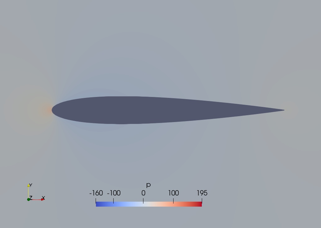
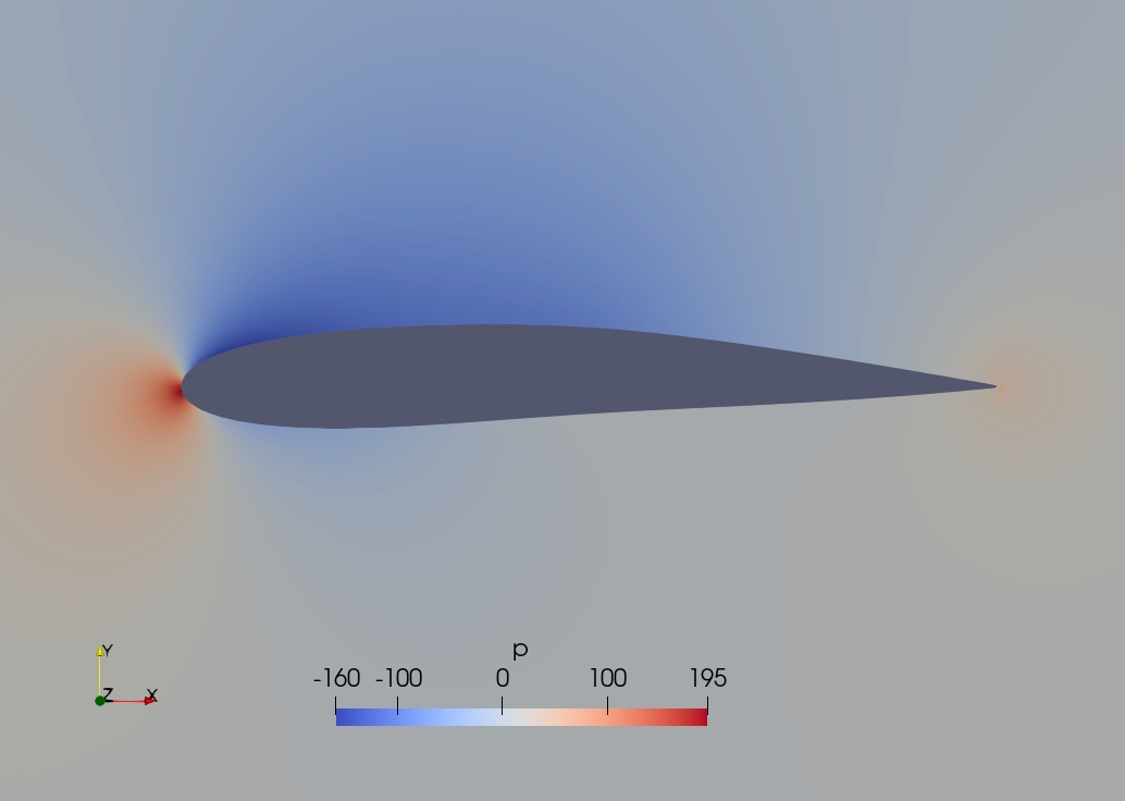
Fig. 1. Pressure contour for the reference (top), baseline (mid), and optimized (bot) designs.
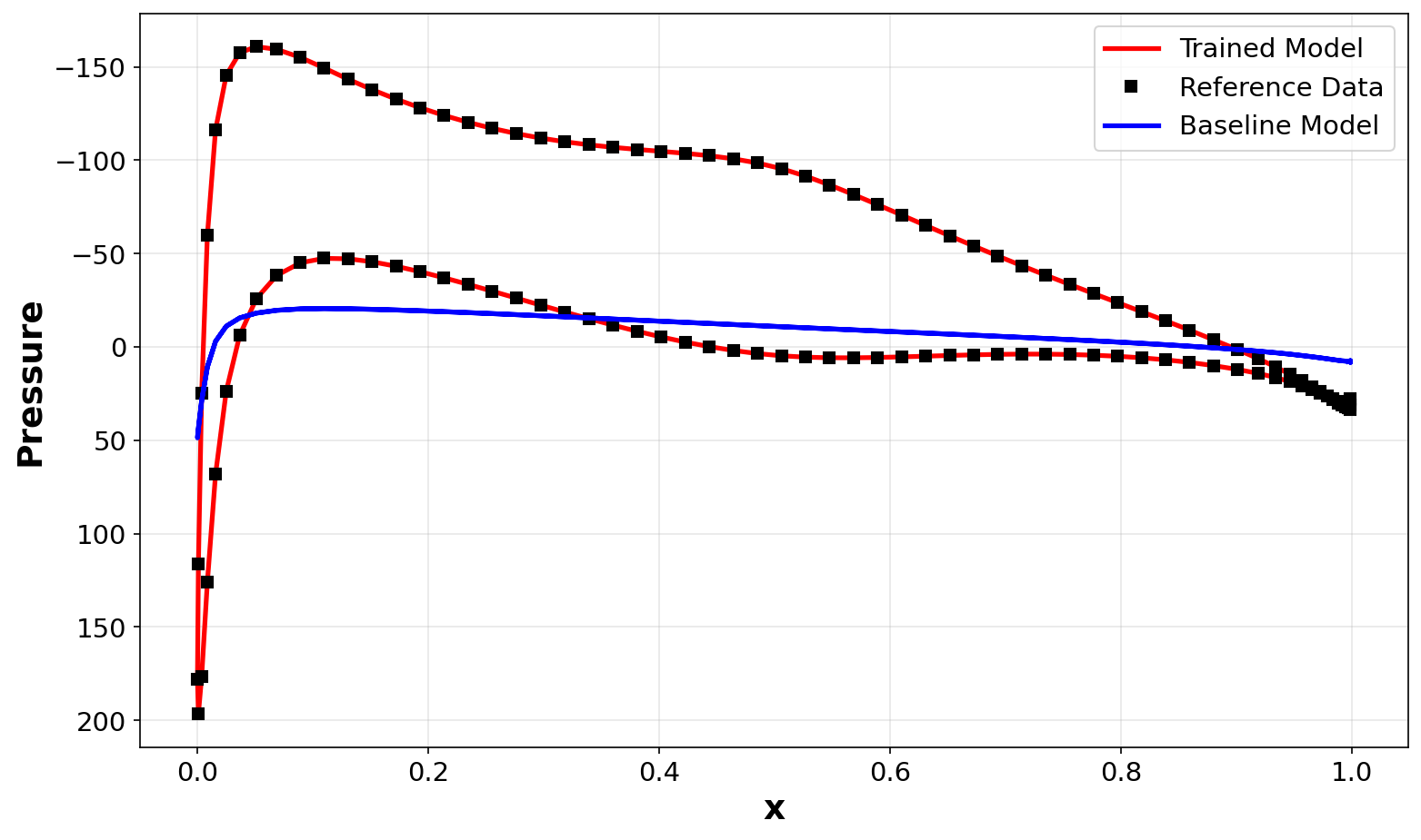
Fig. 2. Wall pressure distributions comparison among the reference, baseline, and optimized designs.
Unsteady flow
The following is a data-assimilation optimization case where we try to find the angle of attack, and airfoil geometry based on time-resolved unsteady pressure data on the NACA0012 airfoil.
Case: Data assimilation optimization (unsteady)
Geometry: NACA0012
Objective function: Time-resolved pressure prediction errors on the airfoil
Design variables: Angle of attack at the far field and the shape of the airfoil
Constraints: None
Reynolds number: 0.6667 million
Mesh cells: 4000
Solver: DAPimpleFoam
To run this case, first download tutorials and untar it. Then go to tutorials-main/NACA0012_DA and run the “preProcessing_unsteady.sh” script to generate the training data.
./preProcessing_unsteady.sh
Then, use the following command to run the optimization with 4 CPU cores:
mpirun -np 4 python runScript_unsteady.py 2>&1 | tee logOpt.txt
The case ran for 100 steps and took about 8 hours using Intel 3.0 GHz CPU with 4 cores. According to “logOpt.txt” and “opt_IPOPT.txt”, the initial and optimized objective functions are 9.4104150e+01 and 1.9374736e-01 with 3 order of reduction.
The animations of the optimization are as follows. We can see that the overall pressure profile and velocity contours agree well with the reference.

Fig. 3. Wall pressure distributions animation, comparing among the reference, baseline, and optimized designs.

Fig. 4. Velocity contour for the reference (top), baseline (mid), and optimized (bot) designs.