Overview
The following is a demonstration of how to perform field inversion using DAFoam. We have selected the periodic hill flow as a demonstrative case. In this tutorial we will show how we can augment the Spalart-Allmaras model using velocity field data for “training”. For the purposes of this tutorial, we will be treating the results from the k-epsilon model as the reference data (for simplicity). We have found the k-epsilon results to be closer to high-fidelity data compared to other RANS models.
Reynolds number: 5,600
Mesh cells: 3,500
Adjoint solver: DASimpleFoam
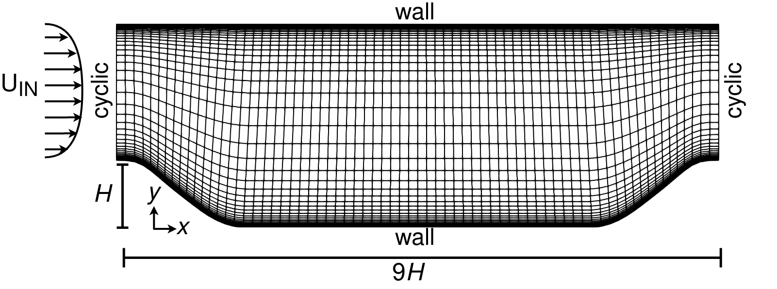
Fig. 1. Periodic hill geometry and mesh.
Run field inversion
To run this case, first download tutorials and untar it. Then go to tutorials-master/PeriodicHill_FieldInversion and run the “preProcessing.sh” script to make a copy of the 0 directory.
./preProcessing.sh
Then, use the following command to run the optimization in serial:
python runScript.py 2>&1 | tee logOpt.txt
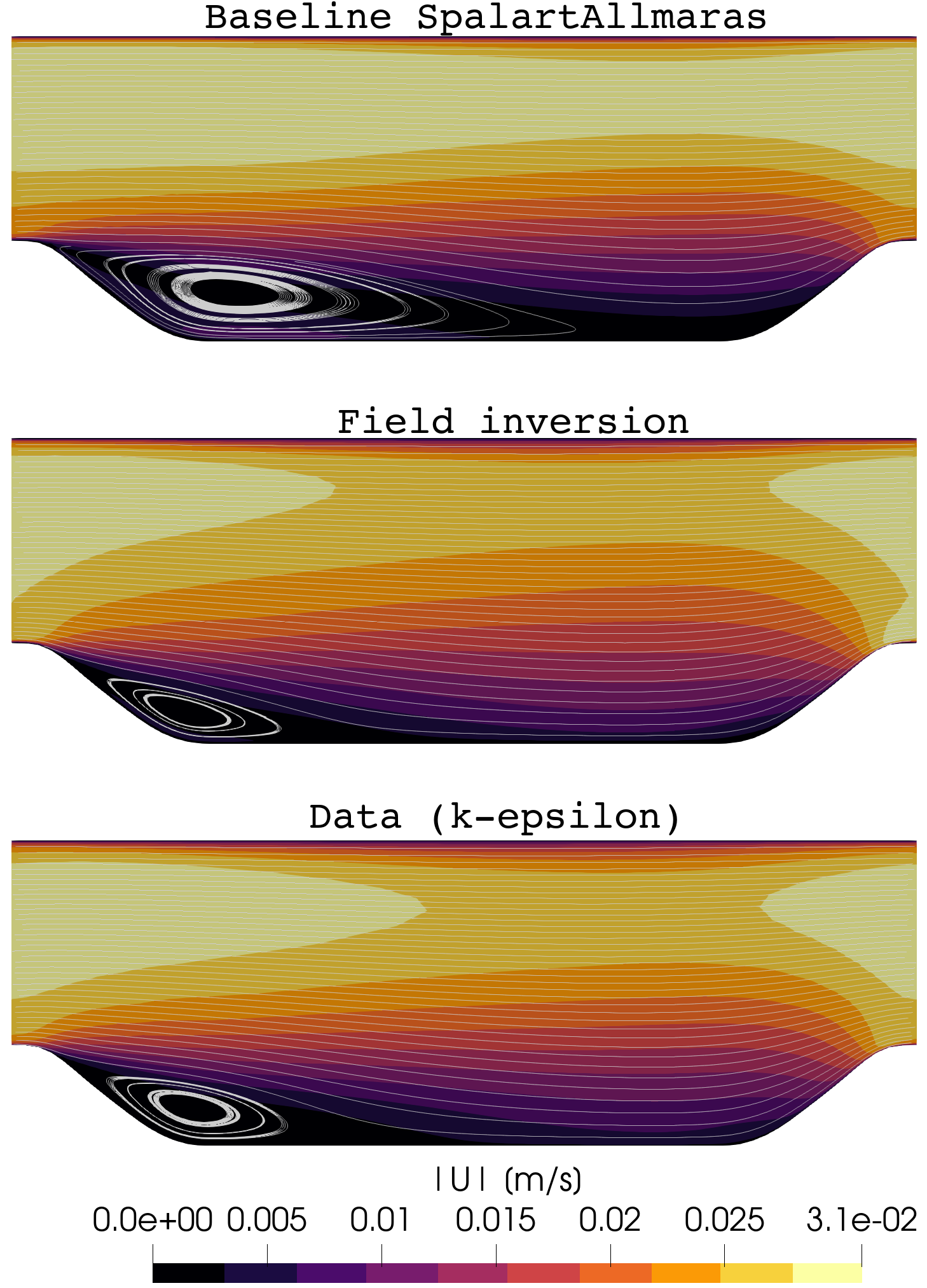
Fig. 2. Velocity magnitude contour.
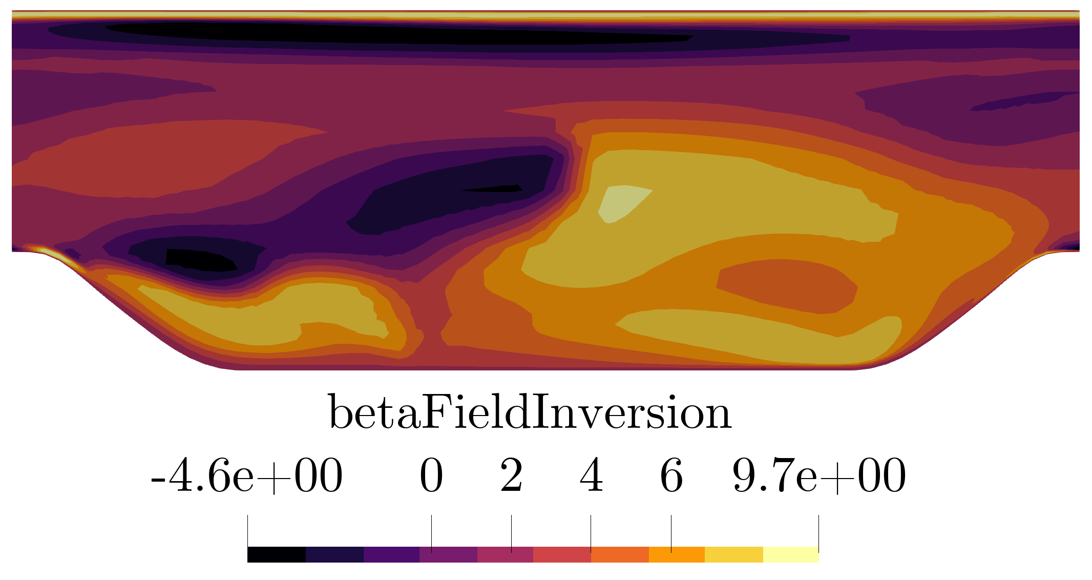
Fig. 3. The optimised corrective field beta.
The case above was terminated after 19 iterations and took approximately 6 hours on Intel 2.40 GHz CPU with 4 cores. The objective function value reduced ~88%.
The field inversion process
Field inversion involves perturbations of the production term in the model transport equation through a spatial field (beta) and the iterative optimisation of this field such that the error between model prediction and data is minimised. Refer to our publication here for the theoretical details.
For those unfamiliar with DAFoam, here is a brief overview of the optimisation process. A high-level Python layer (controlled through runScript.py) is used to set and run the field inversion simulation process outlined in Fig. 4. Specifically, the following parameters are set in a Python script: primal flow solver (i.e. DASimpleFoam); residuals convergence tolerance; the field inversion objective function specialisation and the relevant parameters (so far, the following have been implemented: full fields, velocity profiles, surface pressure and skin friction, and aerodynamic force coefficients); adjoint solver parameters such as state normalisation constants, and the equation solution options; and finally the optimiser and its parameters such as beta field constraints (upper and lower bounds), convergence tolerance, maximum number of iterations, etc.
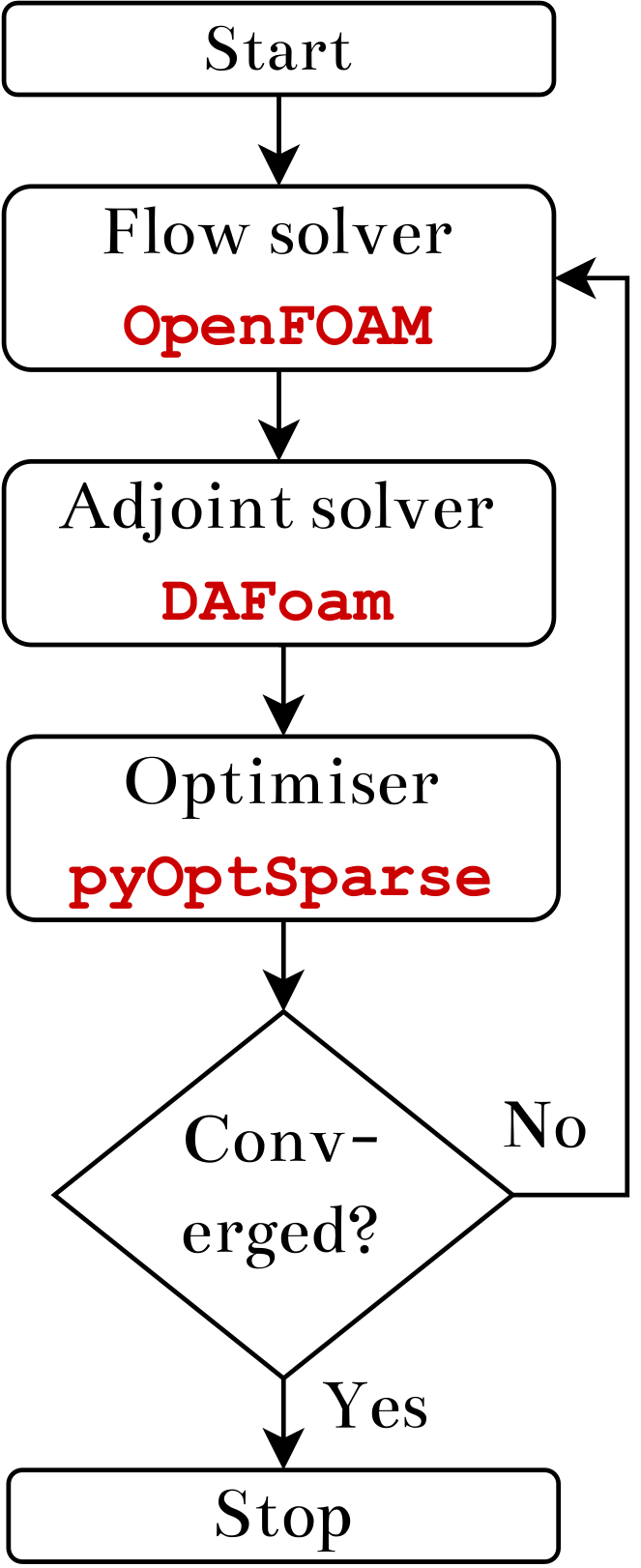
Fig. 4. Field inversion flow diagram.
Selecting turbulence model
This is set in the constant/turbulenceProperties file:
RAS
{
    RASModel        SpalartAllmarasFv3FieldInversion;

    turbulence      on;

    printCoeffs     on;
}
At present the following turbulence models are available for field inversion:
- SpalartAllmarasFv3FieldInversion
- kOmegaSSTFieldInversion (based on OpenFOAM kOmegaSST model, perturbing the omega equation), and
- kOmegaFieldInversionOmega (based on OpenFOAM kOmega model with beta perturbing the omega equation).
Details of the runScript.py
The “runScript.py” for a field inversion is similar to the one used for shape optimization. In other words, we still need to specify a dummy design surface (although we will not move it)
"designSurfaces": ["bottomWall", "topWall", "inlet", "outlet"],
And we need to create a dummy FFD box to cover the dummy design surface and load it to DVGeo,
DVGeo = DVGeometry("./FFD/periodicHillFFD.xyz")
We also need to specify set up a dummy reference axis to make sure we can use global design variable (alpha porosity field)
DVGeo.addRefAxis("bodyAxis", xFraction=0.25, alignIndex="k")
Objective function:
The objective function is normally composed of two terms. A least-squares term and a regularisation term:
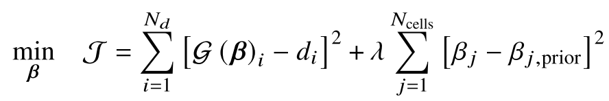
Each term is defined in two sub-dictionaries. The bare minimum entries for each sub-dictionary are:
"obj-term":
{
    "type": "fieldInversion",   # to designate type of objective function
    "source": "boxToCell",      # method for selecting mesh faces to compute the objective function
    "min": [xMin, yMin, zMin],  # min point for source selection
    "max" : [xMax, yMax, zMax], # max point for source selection
    "data": "UData",            # used to designate the objective function specialisation
    "scale": 1,                 # useful when using scaled data (e.g. for U/Uinf, scale = Uinf)
    "addToAdjoint": True,       # want to solve the adjoint equations for optimisation
    "weightedSum": True,        # set to true if you want to normalise the objective function term
    "weight": 1/J0              # where J0 can be the objective function at the 0th optimisation iter
},
For the case above, here is how the objective function is composed.
"FI": {
    "Ux": {
        "type": "fieldInversion",
        "source": "boxToCell",
        "min": [-10.0, -10.0, -10.0],
        "max": [10.0, 10.0, 10.0],
        "data": "UData",
        "scale": 1,
        "addToAdjoint": True,
        "weightedSum": True,
        "weight": 1/J0                          # normalise the objective function
    },
    "beta": {
        "type": "fieldInversion",
        "source": "boxToCell",
        "min": [-10.0, -10.0, -10.0],
        "max": [10.0, 10.0, 10.0],
        "data": "beta",
        "scale": 1e-10,                         # the regularisation constant
        "addToAdjoint": True,
        "weightedSum": False,
    },
},
Design variable (beta) setup:
The following block of code provides design variable (i.e. beta) information to the optimiser, such as initialising it (beta0 = 1) and setting the minimum (keyword: lower) and maximum (keyword: upper) bounds (in this example it is set between -5 and 10).
def betaFieldInversion(val, geo):
    for idxI, v in enumerate(val):
        DASolver.setFieldValue4GlobalCellI(b"betaFieldInversion", v, idxI)

nCells = 3500
beta0 = np.ones(nCells, dtype="d")
DVGeo.addGeoDVGlobal("beta", value=beta0, func=betaFieldInversion, lower=-5.0, upper=10.0, scale=1)
daOptions["designVar"]["beta"] = {"designVarType": "Field", "fieldName": "betaFieldInversion", "fieldType": "scalar"}
Due to the large number of design variables (equal to the number of mesh cells) we are restricted to the IPOPT (open-source and available with DAFoam) and the SNOPT (not open-source, license required) optimisers.
Periodic hill specific inlet pressure gradient:
The following code snippet in the runScript.py is unique to flows where we want to maintain volume-averaged mean velocity, as is required for the periodic hill flow. This is done by adding a finite volume source term to the momentum equation:
"fvSource":{
  "gradP": {
      "type": "uniformPressureGradient",
      "value": 6.634074021107811e-06,       # get this value by running the original OpenFOAM solver
      "direction": [1.0, 0.0, 0.0],
  },
},
Note
The mesh used in this case is very coarse, in order to allow a relatively fast run time. While appropriate for demonstrative purposes, the users are cautioned that these field inversion results are sub-optimal and that better results are achievable with a higher-quality mesh.
Contact
Please note that the field inversion feature in DAFoam is a work in progress. More tutorials, documentation, and features will be added as the work progresses. In the meantime, if you have questions about the tool or would like to collaborate please get in touch: obidar1@sheffield.ac.uk.