This chapter was written by Christian Psenica and reviewed by Ping He.
Learning Objectives:
After reading this chapter, you should be able to:
- Describe the basic file structure of an OpenFOAM simulation (which configuration files in which directories)
- Describe the purpose of each configuration file
- Setup and run a new OpenFOAM simulation
Introduction
Background
OpenFOAM (Open-source Field Operation And Manipulation) is a free open-source finite-volume CFD solver. OpenFOAM is primarily written in C++ and comes with libraries to help facilitate numerical operations on field values. OpenFOAM also has a wide range of utilities for pre- and post-processing, such as mesh generation/quality checks and support for ParaView (for post-process visualization). There are three main branches of OpenFOAM: ESI OpenCFD, The OpenFOAM Foundation, and Extended Project. DAFoam only supports the ESI OpenCFD version, the OpenFOAM version discussed within this document.
Follow Along
This document contains basic information related to setting up OpenFOAM for the steady-state NACA0012 simulation. We will discuss every file within this case in an effort to clarify the various aspects of OpenFOAM.
To help with clarity, below is the file/folder structure for the NACA0012 case. As a general overview: 0.orig contains boundary conditions and initial field values, constant handles flow properties (such as turbulence model and fluid modeling parameters), and system controls the numerical discretization, equation solution parameters, etc. This document serves as detailed documentation for these directories.
- 0.orig               // initial fields and boundary conditions
- constant             // transport/ turbulence property information and mesh files
- system               // flow discretization, simulation run parameters, solver settings etc.
- clean                // script to clean and reset case to default
- paraview.foam        // dummy file used by ParaView to load results
- run                  // script to execute simulation
These steps will be elaborated on in the coming sections with particular emphasis on the 0.orig, constant, and system directories. It is intended that the user read this documentation carefully to gain a basic understanding of OpenFOAM. It is also recommended to follow along in the tutorial cases to recreate the simulation and post-process using ParaView (Don’t have ParaView? Download it here!).
1. Boundary and Initial Conditions - 0.orig
The 0.orig directory contains both the boundary conditions and the initial field values for the simulation. For clarity purposes, it should be noted here that this simulation contains a wing boundary (wall), an inout boundary (far field domain), and two symmetry planes (one for either side of the airfoil) as denoted by Fig.1.
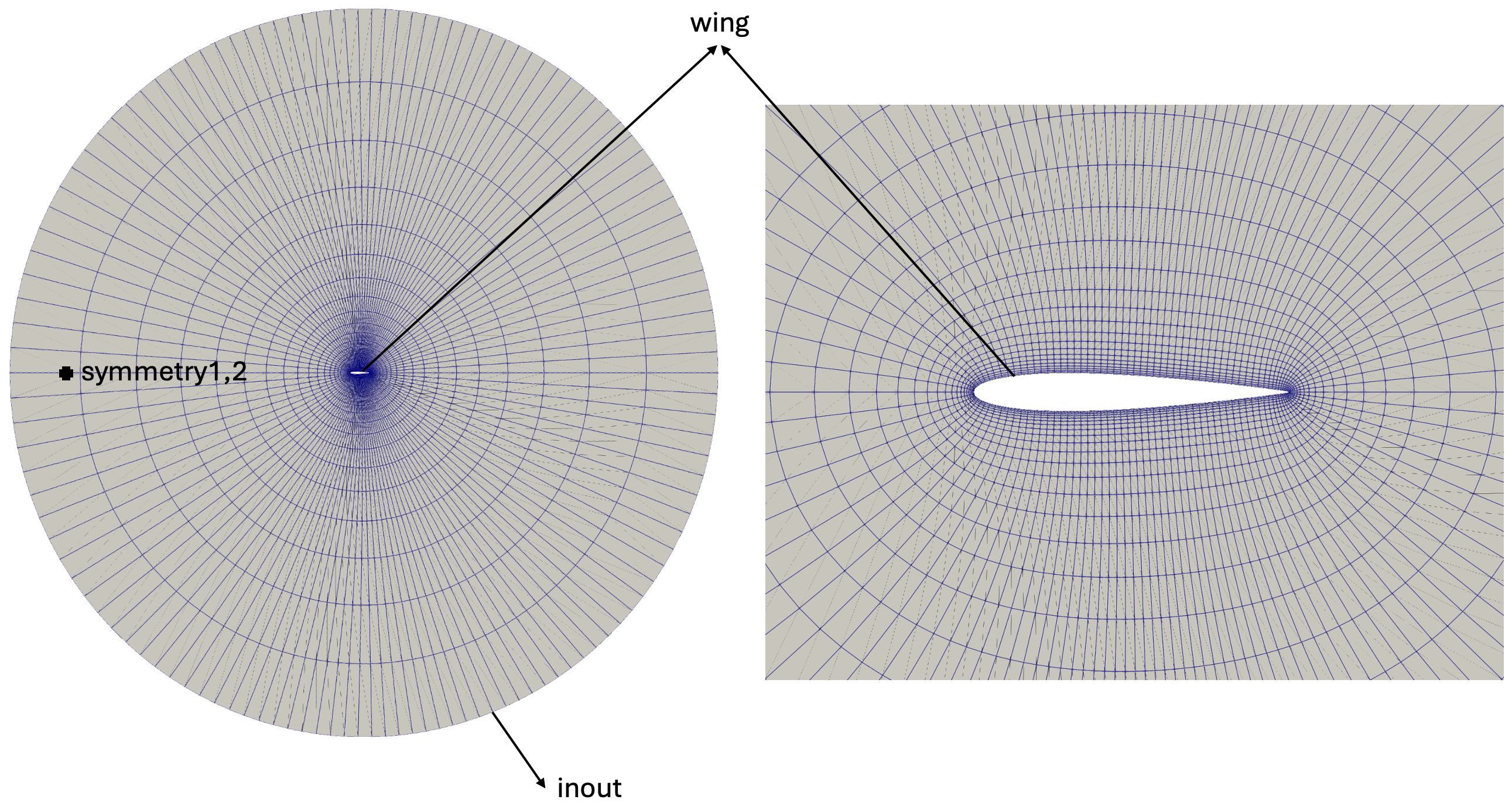
Fig.1 Labeled boundaries of the OpenFOAM NACA0012 case
For this NACA0012 case, we can expand the 0.orig directory to see which field values have specified boundary conditions:
|-- 0.orig        // directory containing BCs
  |-- nut         // turbulent kinematic viscosity
  |-- nuTilda     // modified turbulent viscosity
  |-- p           // pressure
  |-- U           // velocity
As a note: we name this folder 0.orig. This is not a necessity; OpenFOAM needs this file to be named 0 at the start of the simulation. Hence, in the run script, we have the line cp -r 0.orig 0. Since we may modify the files in the 0 folder later in simulations/optimizations, having a 0.orig backup folder will ensure reproducibility. To avoid confusion, as a motivated reader may notice that various sources use either 0 or 0.orig naming conventions, we leave the name of this folder as 0.orig and note the distinction here.
1.1 The dimensions and internalField
As a preface to the following boundary conditions discussed, we will clarify a couple of entries found in all boundary condition files: dimensions and internalField.
When entering values for both boundary conditions and internalField, it is important to be mindful of the units used, as they are not all constant. Though OpenFOAM’s default is SI units, the derived units are based on which solver is used. For example, if using the simpleFoam solver (the incompressible flow solver we will use for the NACA0012 case), pressure is expected to be the kinematic pressure, which is measured in $m^2/s^2$. However, if using rhoSimpleFoam (compressible flow solver), then pressure is measured as thermodynamic pressure, measured in Pascals ($N/m^2 = kg/(m*s^2)$). The exact units used are specified by the dimensions key in 0.orig/. Using the same 0.orig/U from the NACA0012 case, we can see the dimensions used for velocity are dimensions [0 1 -1 0 0 0 0];. This is, as one would suspect, $m/s$. But looking at solely the dimensions key, this may not be so obvious. However, it is in fact very simple:
dimensionsUsed  [Mass Meter Second Kelvin Mole Ampere Candela]

dimensions      [0 1 -1 0 0 0 0];
The dimensions key is a list containing 7 numbers. Each (non-zero) number in dimensions denotes which unit is being used, corresponding to the entries in dimensionsUsed (this key is for an example, it is not an actual key used in OpenFOAM). A zero indicates that the unit is not being used. The value of the actual (non-zero) numbers gives the exponent on the unit. So an entry of [0 1 0 0 0 0 0] gives meter ($m$). However, [0 2 0 0 0 0 0] indicates $m*m = m^2$ and so on. A negative sign before the number indicates a negative exponent. Knowing this, it becomes clearer to see which units are expected. As an example, the kinematic pressure, $m^2/s^2$, would be dimensions [0 2 -2 0 0 0 0].
Lastly, the internalField key is used as an initial condition to the problem and should be assigned with care. Field values such as pressure, temperature, velocity etc. can be easily assigned by the user and depend on what the user wants to simulate. The calculations for turbulent fields (such as nuTilda, k, epsilon etc.) are beyond the scope of this beginner user guide and we encourage the motivated reader to see the advanced OpenFOAM user guide for a breakdown on these calculations.
1.2 Velocity (U)
For the NACA0012, the fluid flow is 10 m/s in magnitude at an angle of attack of ~5.14 degrees:
dimensions      [0 1 -1 0 0 0 0];          // dimensions for velocity

internalField   (9.9598 0.89575 0);        // velocity components at AOA = 5.139186 degreees

boundaryField
{
    wing                                   // patch name to apply BC to
    {
        type            fixedValue;        // type of BC, could use noSlip
        value           uniform (0 0 0);   // value at boundary
    }

    symmetry1
    {
        type            symmetry;          // symmetry type, nothing else to specify
    }

    symmetry2
    {
        type            symmetry;
    }

    inout
    {
        type            inletOutlet;       // handles reverse flow at outlets
        inletValue      $internalField;
        value           $internalField;
    }
}
The wing boundary takes on a fixedValue uniform (0 0 0); condition. This enforces a no-slip boundary condition at the wall. This is also equivalent to using type noSlip; on the wing (either will work). The symmetry boundary condition will ensure an identical flow field over the two symmetry planes present (this is consistent for all field values specified in this section). The inletOutlet boundary condition automatically applies fixedValue when the flow enters the simulation domain with the values given by the inletValue key, and zeroGradient when the flow exits the domain. Here, the user can use $internalField to specify the far field domain conditions: prescribe the same as the internalField value defined above (i.e., uniform (9.9598 0.89575 0)). The value key for the inout patch prescribes an initial value for this patch, and this value will be automatically updated (depending on whether the flow enters or leaves the domain) when the simulation starts.
1.3 Pressure (p)
Since this is an incompressible flow simulation, the pressure is given as the kinematic pressure ($m^2/s^2$). For incompressible flow solvers, the pressure value is calculated as the relative pressure with respect to a reference value (e.g., 101325 Pa), so here we prescribe 0 (internalField uniform 0;). NOTE: for compressible flow solvers, the pressure value is the absolute pressure value, so we would need to prescribe 101325 instead.
dimensions      [0 2 -2 0 0 0 0];

internalField   uniform 0;

boundaryField
{
    wing
    {
        type            zeroGradient;
    }

    symmetry1
    {
        type            symmetry;
    }

    symmetry2
    {
        type            symmetry;
    }

    inout
    {
        type            outletInlet;
        outletValue     $internalField;
        value           $internalField;
    }
}
Wall boundaries (such as the wing) typically use a zeroGradient pressure boundary condition type. As mentioned previously, the symmetry planes always receive the symmetry type boundary condition (in the following sections, 1.4-1.8 we will omit discussion of this in an effort to reduce redundancy). The pressure far field domain uses an outletInlet boundary condition, where inlets are zeroGradient while outlets are fixedValue.
1.4 Turbulent Kinematic Viscosity (nut)
The following sections (1.4-1.5) are all turbulence field values. It is not uncommon, though not all the time necessary, to use wall functions for these values (mesh y+ > 30). For now, we will just state the use of wall functions and point the reader to the advanced OpenFOAM user guide for in-depth details on wall functions and their applications within OpenFOAM. The discussion for these turbulent fields will also be brief, as the types of boundary conditions specified largely remain unchanged aside from the wing boundary. For the turbulent viscosity, we use the wall function nutUSpaldingWallFunction. Similar as before, this is a wall function specifically designed for the nut turbulent field.
dimensions      [0 2 -1 0 0 0 0];

internalField   uniform 4.5E-5;

boundaryField
{
    wing
    {
        type            nutUSpaldingWallFunction;
        value           $internalField;
    }

    symmetry1
    {
        type            symmetry;
    }

    symmetry2
    {
        type            symmetry;
    }

    inout
    {
        type            calculated;
        value           $internalField;
    }
}
For this field however, we switch the inout boundary condition type to calculated. This naturally raises two questions: what is a calculated boundary condition type, and why use this type versus inletOutlet such as the other turbulent fields?
Put simply, nut is a turbulent field which is not solved for directly, its value depends on (calculated from) other field values. Due to this, we do not want to assign a value to this field. We want OpenFOAM to solve for it throughout the simulation process. Therefore, we apply the calculated boundary condition type to tell OpenFOAM to solve for this field value rather than read in a user-prescribed value on the boundary.
1.5 Modified Turbulent Viscosity (nuTilda)
The modified turbulent viscosity is not a calculated field, meaning OpenFOAM solved for it directly, hence the inout boundary uses inletOutlet again. This field is specific to the Spalart-Allmaras turbulence model (which we use for the NACA0012 case) and is, in some cases, referred to as the Spalart-Allmaras variable. However, a wall function is not used for this field value on our wall boundary, wing. Rather, we always assign a zero value to the wall for nuTilda.
dimensions      [0 2 -1 0 0 0 0];

internalField   uniform 4.5e-05;

boundaryField
{
    wing
    {
        type            fixedValue;
        value           uniform 0.0;
    }

    symmetry1
    {
        type            symmetry;
    }

    symmetry2
    {
        type            symmetry;
    }

    inout
    {
        type            inletOutlet;
        inletValue      $internalField;
        value           $internalField;
    }
}
2. Transport, Turbulence, and Mesh Properties - constant
The constant directory contains information related to turbulence and transport properties (and in other cases, thermophysical properties). Additionally, the mesh used for the simulation resides in constant/polyMesh. The file structure for the NACA0012 case is shown below for clarity:
|-- constant                 // directory containing mesh, turbulence model, and transport properties
  |-- polyMesh               // directory containing the mesh
    |-- boundary             // list of boundaries and associated mesh cells
    |-- faces                // list of cell faces
    |-- neighbour            // list of neighbour cell labels
    |-- owner                // list of owner cell labels
    |-- points               // vectors describing mesh cell verticies
  |-- transportProperties    // fluid transport parameters
  |-- turbulenceProperties   // turbulence parameters
2.1 Mesh Files (polyMesh)
The mesh is user-generated and can be generated using various methods/ tools. This can be done using third party programs or using OpenFOAM’s built in tools (such as snappyHexMesh). For the NACA0012 case, the mesh is already generated and ready to use for the simulation.
For the discussion of the polyMesh directory, we will limit this section to showing the most pertinent file, boundary. This is the file most viewed in the polyMesh directory, and shows the various boundaries generated during the meshing process. The remaining files (faces, neighbour, owner, and points) all contain organizational data on the mesh. Although it is possible to modify a few select entries within the boundary file without breaking the mesh (a topic left for the advanced OpenFOAM user guide) it is highly recommended to never try and make manual adjustments to the remaining files. Although possible in theory to make modifications to these files successfully, it is very error-prone and not an intended feature. If the physical mesh needs to be adjusted, the best practice is to always regenerate the mesh and have OpenFOAM modify these files for you. Below we can see the boundary file for our NACA0012 case:
4                                       // total number of boundaries in mesh
(
    symmetry1                           // name of boundary
    {
        type            symmetry;       // type of boundary
        inGroups        1(symmetry);
        nFaces          4032;
        startFace       7938;
    }
    symmetry2
    {
        type            symmetry;
        inGroups        1(symmetry);
        nFaces          4032;
        startFace       11970;
    }
    wing
    {
        type            wall;
        inGroups        1(wall);
        nFaces          126;
        startFace       16002;
    }
    inout
    {
        type            patch;
        nFaces          126;
        startFace       16128;
    }
)
From the boundary file, we first notice the number 4. This number indicates the total number of boundaries defined in our mesh. As we saw from Sec.1, we indeed have four boundaries: two symmetry planes, the wing itself, and the far field domain. Each one of these boundaries is defined here. Within each boundary entry, there is an accompanying dictionary providing extra information for OpenFOAM regarding the boundary. The type key tells OpenFOAM what type of boundary we have. As expected, the symmetry planes are type symmetry, the wing itself is a wall boundary, and the far field is a patch (allowing fluid to flow through). Similar boundary types will be grouped together in OpenFOAM for organization, hence the inGroups key. nFaces tells OpenFOAM how many cell faces are contained within the given boundary. startFace tells OpenFOAM which cell is the first cell making up a boundary. All mesh cells in OpenFOAM are numbered, and these two keys help OpenFOAM identify boundaries. NOTE: the patch names between the fields in the 0 folder (e.g., 0/U) and constant/polyMesh/boundary need to be consistent.
2.2 transportProperties
The transportProperties file contains fluid specific properties which help define what kind of fluid is being simulated (most common air but of course other fluids can be modeled such as water or various gases). In a general sense, transportProperties is not the only file containing fluid parameters. For example, thermophysicalProperties also contains compressible fluid parameters but is not included in our NACA0012 case as this simulation considers only incompressible flow.
transportModel Newtonian;  // transport model being used

nu    1.5e-5;              // dynamic viscosity
Pr    0.7;                 // Prandtl number
Prt   0.85;                 // turbulent Prandtl number
The first entry tells OpenFOAM which transport model to use. The Newtonian transport model used in the NACA0012 case assumes a constant dynamic viscosity (nu). Hence, the following entry, nu, where we give this constant value for OpenFOAM to use. The value used here, $1.5e-5$ is a typical value used for modeling air.
The following two entries are the Prandtl number and turbulent Prandtl number. The Prandtl number is a dimensionless quantity, a ratio of momentum diffusivity (kinematic viscosity, $\nu$) to thermal diffusivity ($\alpha$). The Prandtl number alone does not help describe fluid behavior for turbulent flow, hence the inclusion of the turbulent Prandtl number, Prt. Together, these quantities help identify if momentum diffusivity or thermal diffusivity dominates the fluid flow for both laminar and turbulent flow. Values for Pr Prt of 0.7 and 0.85, respectively are typical for modeling air.
2.3 turbulenceProperties
The turbulenceProperties file informs OpenFOAM of how users wish to model turbulence. We can see how turbulence modeling is defined below in this file:
simulationType RAS;                     // type of simulation to run
RAS                                     // dictionary containing turbulence model parameters
{
    RASModel        SpalartAllmaras;    // specific turbulence model to use
    turbulence      on;                 // whether to model turbulence or only laminar flow
    printCoeffs     off;                // whether to print turbulence model coefficients
}
For our NACA0012 case, we elect a Reynolds Averaged Simulation (RAS). There are other options available for the user which are outlined in the advanced OpenFOAM user guide. Within the RAS dictionary we choose to use the SpalartAllmaras turbulence model. This is a very commonly used one-equation (solves a single transport equation) model using the ‘Spalart-Allmaras variable’, nuTilda. We elect this model typically due to it’s simplicity and low computational cost. An exhaustive discussion on turbulence models in OpenFOAM can be found in the advanced OpenFOAM user guide.
The following entry, turbulence on; tells OpenFOAM to model turbulent flow, not just laminar flow. printCoeffs off; refers to the coefficients used in the Spalart-Allmaras turbulence model equation. These coefficients are beyond the scope of this user guide, and for the purposes of our NACA0012 case, we do not need to adjust these coefficients for this turbulence model hence we do not print these coefficients. For more advanced applications, these coefficients may need to be adjusted which would make printCoeffs on; a sensible entry.
3. Flow Discretization, Simulation Run Parameters, and Solver Settings - system
The system directory is home to most simulation parameters. Within this directory, we specify things such as simulation run time, how to decompose the domain (only needed for running a simulation in parallel), as well as solver settings.
|-- system               // directory global simulation parameters
  |-- controlDict        // define solver, and simulation runtime parameters
  |-- decomposeParDict   // decompose the simulation domain to run in parallel
  |-- fvSchemes          // solution schemes
  |-- fvSolution         // iterative solution and algorithm parameters
3.1 Simulation Runtime Parameters (controlDict)
Below we can see the various inputs in controlDict. The inputs from the application key to runTimeModifiable are required by OpenFOAM to run the simulation. The following block of code, the functions dictionary, is optional.
Since we seek to run a steady-state, incompressible flow case, we elect the simpleFoam solver for the application key. To specify how long we want the simulation to carry out (simulation time), we start the simulation at startTime 0; and tell OpenFOAM to start from this time (startFrom startTime;). We also need to tell OpenFOAM to stop at our specified end time. We use the stopAt endTime; entry for this and prescribe endTime 1000; (where this time is measured in seconds). The time step, deltaT is set to 1 second (this is fine and common practice for steady-state simulations, but for an unsteady simulation we would need a much smaller time step to maintain a stable simulation).
The writeControl key tells OpenFOAM how to measure when to write field values to the disk. Here we prescribe timeStep, effectively telling OpenFOAM we wish to write data at some increment based on the time step of the simulation. This is then a coupled entry with writeInterval; we only need the data at the end of the simulation so we set the writeInterval to 1000 seconds, matching our endTime. Combining writeControl and writeInterval, OpenFOAM understands this to be: “write the data every 1000 time steps”.
The purgeWrite key is an integer representing the limit on the number of time directories stored during a simulation. Here we disable this entry by passing a value of zero. If, for example, this entry were two, then only the latest two time directories will saved throughout the simulation (where old time directories are over written by new ones). For large cases, depending on the application, this can save a lot of storage. Additionally, we turn use writeCompression on; which tells OpenFOAM to store data in compressed files (gzip compression) rather than uncompressed (another method to save storage). We save our data in a human readable format, writeFormat ascii;, though we may also specify to store data as binary. When storing this data, we can choose how many decimal places to record. Here we choose 8: writePrecision 8;. This is the same where recording simulation time (timePrecision 8;). Lastly, we use timeFormat general; which instructs OpenFOAM to use general naming conventions for time directories.
application         simpleFoam;    // solver to use
startFrom           startTime;     // where to start simulation from
startTime           0;             // what time the simulation starts at (0 seconds)
stopAt              endTime;       // when to end simulation
endTime             1000;          // end time of simulation
deltaT              1;             // timeStep
writeControl        timeStep;      // when to check for writing data
writeInterval       1000;          // how often to write
purgeWrite          0;             // number of time directories to keep (0 to disable)
writeFormat         ascii;         // ascii or binary data format
writePrecision      8;             // precision in written data
writeCompression    on;            // compress written data using gzip compression
timeFormat          general;       // format names of time directories
timePrecision       8;             // precision used for simulation time

functions
{
    aeroForces
    {
        type            forceCoeffs;        // type of function
        libs            ("libforces.so");   // library for function
        patches         (wing);             // patch to calculate forces on
        p               p;                  // pressure field to use
        U               U;                  // velocity field to use
        rho             rhoInf;             // density field to use
        rhoInf          1.225;              // SSL density
        pRef            0;                  // reference pressure
        porosity        no;                 // model porosity effects?
        liftDir         (0 1 0);            // lift direction
        dragDir         (-1 0 0);           // drag direction
        pitchAxis       (0 0 1);            // pitch axis
        CofR            (0.025 0 0);        // rotation axis for momentum calculation
        magUInf         10;                 // magnitude of far field velocity
        lRef            0.1;                // reference length
        Aref            0.1;                // reference area
        log             true;               // write to log file
        writeControl    timeStep;
        writeInterval   1000;
    }
}
The next block of code is functions. In OpenFOAM, when the user wants to add some type of calculation, this is typically done within controlDict. As is typical with wing (airfoil for our NACA0012 simulation) cases, we want to simulate this wing in order to get aerodynamic data from it. One way we can do this is with the function aeroForces. The name aeroForces is specified by the user. For incompressible steady-state simulations, these entries can remain mostly unchanged from one case to another. However, there are a few pertinent entries to discuss. We must tell OpenFOAM which patch we want to calculate the aerodynamic forces for via patches (wing);. Additionally, we must prescribe the lift and drag direction in accordance with our global coordinate system. Here, we have a lift acting in the positive y-direction. Drag is in the positive x-direction (though multiplied by negative one to give the force acting on the wing). Our pitch axis is the z axis. As we are modeling an airfoil instead of a wing, we use Aref = lRef = 0.1 which is our chord length. For a wing case, Aref should be the planform area whereas lRef is the mean aerodynamic chord.
3.2 Decomposition of Domain (decomposeParDict)
Oftentimes these CFD simulations last a very long time. To help speed up the process, we can run the job in parallel, splitting up the simulation over multiple computer processors. This will greatly decrease the real-world run time of the simulation. To do this, we use decomposeParDict:
numberOfSubdomains  4;         // number of processors to split domain over
method              scotch;    // method for decomposition (splitting) domain
As can be seen by the above block, there are very few inputs to this file. Since the NACA0012 case is very light weight (coarse mesh in a steady simulation) we choose to only split (decompose) the domain into 4 distinct parts. These parts will be distributed over 4 processor cores when running. To see this, when running the case, you will find directories processor0 processor1 ... processor3 in your working directory. This is controlled by the numberOfSubdomains entry. For our NACA0012 case, and for most cases, we can choose a very simple and automatic decomposition algorithm, method scotch;. This method is very common to use as it is simple (requires no other entries), and handles everything automatically. There are other decomposition methods available, such as hierarchical, which will require a coeffs entry in decomposeParDict. This method is not needed for now, but for the motivated reader there are a few additional notes in decomposeParDict regarding this.
3.3 Numerical Schemes (fvSchemes)
fvSchemes delves into the particular numerical schemes used to solve the Navier-Stokes equations, particularly how to handle derivatives. An in-depth analysis of the parameters found in fvSchemes is covered in the advanced OpenFOAM user guide. For this user guide, we will mostly focus on the basic ideas and define the various dictionaries within fvSchemes. Below is the fvSchemes for our NACA0012 simulation:
// time derivative scheme
ddtSchemes
{
    default                                       steadyState;
}

// gradient schemes
gradSchemes
{
    default                                       Gauss linear;
}

// divergence schemes
divSchemes
{
    default                                       none;
    div(phi,U)                                    bounded Gauss linearUpwindV grad(U);
    div(phi,T)                                    bounded Gauss upwind;
    div(phi,nuTilda)                              bounded Gauss upwind;
    div(phi,k)                                    bounded Gauss upwind;
    div(phi,omega)                                bounded Gauss upwind;
    div(phi,epsilon)                              bounded Gauss upwind;
    div((nuEff*dev2(T(grad(U)))))                 Gauss linear;
}

// point to point interpolation scheme
interpolationSchemes
{
    default                                       linear;
}

// laplacian scheme
laplacianSchemes
{
    default                                       Gauss linear corrected;
}

// component of gradient normal to surface
snGradSchemes
{
    default                                       corrected;
}

// wall disctance computation method
wallDist
{
    method                                        meshWave;
}
We first take note of ddtSchemes. As we want a steady-state simulation, we select steadyState for our time derivatives. In an unsteady case, it is common to use entries such as euler or backward. The steadyState entry will zero out time derivatives (will not compute them).
Following this, we specify our gradient schemes (how we interpolate values for the gradient terms). We specify using default Gauss linear;, which applies Gauss linear for all gradient terms. For some background, Gauss denotes the standard finite volume discretization using Gaussian integration which interpolates from cell centers to cell faces (at the center location on the face). Gauss linear is a second order accurate scheme.
The divSchemes dictionary is used to calculate divergence terms. It is generally not recommended to use just one exact type of divergence scheme as different terms are best solved using different methods. Hence, we elect no default option: default none;. The following six terms, div(phi,U) to div(phi,epsilon) represent the divergence schemes for convective terms. In this case, phi represent $\phi=\rho U$. For these terms, with the exception of div(phi,U), we use bounded Gauss upwind;, a first-order bounded accurate scheme which uses upwind differencing. For div(phi,U) we choose bounded Gauss linearUpwindV grad(U); which is second order accurate using linear upwind differencing. The V term denotes a specialized version of the scheme designed for vector fields and the grad(U) is used for correction. For these schemes, the bounded keyword helps prevent unphysical oscillations/overshoot in the solution. Lastly, we specify div((nuEff*dev2(T(grad(U))))) which is the viscous stress divergence term (the diffusive term in the momentum equation of the Navier-Stokes equations). For this term we apply Gauss linear; which uses central differencing (second order accurate).
The interpolationSchemes dictionary is used as a general setting for interpolating values, typically from cell centers to face centers. For this we use linear which is central differencing. The laplacianSchemes dictionary contains solution schemes for our Laplacian (divergence of gradient) terms. Here we apply a default setting of Gauss linear corrected. These terms tend not to be as tricky (in terms of stability) as our divergence terms (divSchemes). Hence, we are able to apply a default setting.
The next dictionary, snGradSchemes, pertains to surface normal gradients. This dictionary computes surface normal gradients which are required to compute a Laplacian term using Gaussian integration. As this calculation requires orthogonality at the wall to maintain second order accuracy, we must be careful with our default setting. If the mesh maintains high orthogonality, then we can specify default orthogonal. This is fairly uncommon, most applications will not have a very high orthogonality at the wall, such as our NACA0012 mesh. To circumvent this, we use default corrected; which applies a correction for orthogonality to help maintain second order accuracy. The final entry is the wallDist dictionary. This dictionary handles calculating the distance to the nearest patch for all cells and boundaries. For this we use method meshWave;. This method works best for regular, undistorted meshes (low skewness, high orthogonality). For most cases, however, this method works well and is employed here (there is an optional correction term that can be added correctWalls true; which can correct the calculation for skewed/distorted meshes but this option is not needed for our NACA0012 case).
3.4 Iterative Solution and Algorithm Parameters (fvSolution)
In fvSolution, the equation solvers, their associated tolerances, and algorithms are defined. Below is the fvSolution for the NACA0012 case:
// dictionary for SIMPLE algorithm
SIMPLE
{
    consistent                         false;
    nNonOrthogonalCorrectors           0;
}

// solver settings and tolerances
solvers
{
    "(p|p_rgh|G)"
    {

        solver                         GAMG;
        smoother                       GaussSeidel;
        relTol                         0.1;
        tolerance                      0;
    }

    "(U|T|e|h|nuTilda|k|omega|epsilon)"
    {
        solver                         smoothSolver;
        smoother                       GaussSeidel;
        relTol                         0.1;
        tolerance                      0;
        nSweeps                        1;
    }
}

// relaxation factors
relaxationFactors
{
    fields
    {
        "(p|p_rgh)"                         0.30;
    }

    equations
    {
        "(U|T|e|h|nuTilda|k|epsilon|omega)" 0.70;
    }
}
Similar to fvSchemes, most higher level details of this file are best suited and covered in the advanced OpenFOAM user guide. Here we define the dictionaries and discuss the main ideas behind them.
The first dictionary, SIMPLE, where we define both consistent and nNonOrthogonalCorrectors. There are two variations of the SIMPLE algorithm in OpenFOAM: SIMPLE and SIMPLEC. The default algorithm, what we use for the NACA0012 case, is SIMPLE. We can specify SIMPLEC by setting consistent yes;. Additionally, we set nNonOrthogonalCorrectors 0;. This entry controls the extra amount of iterations performed in the unsteady version of SIMPLE algorithm to help account for non-orthogonal meshes. For steady-state simulations, using zero correction is fine.
The following dictionary is the solvers dictionary. In all sub-dictionaries, we specify a solver and smoother to begin. The details for solvers and smoothers are beyond the scope of this user guide (reference the advanced OpenFOAM user guide). The quantities here of most importance for now are the tolerances. For all sub-dictionaries, we specify a tolerance that we wish OpenFOAM to reach in the solution. A tolerance of 0 is very tight, and difficult to meet (taking machine precision to be zero). We can relax this requirement by specifying relTol. A relTol, which stands for relative tolerance, gives how much we want our baseline residual to drop. So a relative tolerance of 0.1 gives that when the residual has dropped by a factor of 10, the solution has sufficiently converged. Note that we need to only converge 1 order for each iteration because the flow solver is nonlinear; there is no need to converge very tightly for each inner linear equation solution. It should be noted at this point that we define different solver settings for various field values (i.e. not all field values use the same solvers/settings, we use 2 total sub-dictionaries to define different solvers/settings). As was the case with fvSchemes; simply put, different field values benefit from particular solvers/settings (this topic again, covered in the advanced OpenFOAM user guide).
Lastly we define relaxation factors within the relaxationFactors dictionary. These factors can help converge the solution much faster and more robust. We define two sub-dictionaries: fields and equations. The fields relaxation factors help stabilize the pressure calculations after solving the equation for that field whereas the equations relaxation factors are applied to the actual linear equation solution of that field. The values used, 0.3 and 0.7, are fairly typical/standard and can work well for most cases meaning that often times, these do not have to be adjusted.
4. run, clean, and paraview.foam
This final section pertains to the last 3 files that we are yet to cover: run, clean, and paraview.foam. These files are simple and pertain to running the case and post-processing.
clean
The clean (bash) script is used to delete all generated files/directories after running a simulation. This is a bash script, which only uses the rm -rf command to delete these generated files/directories, and should be executed before re-running the simulation. Not running this executable before re-running can often times cause OpenFOAM to terminate the simulation right away.
paraview.foam
The paraview.foam file is a dummy file used by ParaView. It is an empty file that the user loads into ParaView to visualize the results. When the user loads this file into ParaView, ParaView will automatically extract all data from the case for post-processing.
run
The run (bash) script is used to actually begin the simulation:
source $WM_PROJECT_DIR/etc/bashrc                   # source OpenFOAM
cd "${0%/*}" || exit                                # run from this directory
. ${WM_PROJECT_DIR:?}/bin/tools/RunFunctions        # tutorial run functions
#------------------------------------------------------------------------------

# whether to run job in parallel or not
parallel=true

# copy initial field/BCs
cp -r 0.orig 0

# run simulation
if [ "$parallel" = true ]
then

    runApplication decomposePar
    runParallel $(getApplication)
    runApplication reconstructPar
    rm -rf processor*

else

    runApplication $(getApplication)

fi
This script sources OpenFOAM and its run functions to begin. $WM_PROJECT_DIR is an environment variable that points to the OpenFOAM installation to help easily source OpenFOAM. Hence, we can source OpenFOAM by running source $WM_PROJECT_DIR/etc/bashrc. In a similar manner we also source OpenFOAM’s run functions (such as runApplication and runParallel seen later in the file) by running . ${WM_PROJECT_DIR:?}/bin/tools/RunFunctions. Running cd "${0%/*}" || exit tells OpenFOAM to run within the directory that the case resides, not necessarily the directory from which the run script is executed. This is not a needed line, but it offers some convenience to the user.
It is recommended to run this NACA0012 case in parallel as that will speed up the time it takes for the simulation to complete. However, here we have included this as an option to show the user how a case can be run in parallel or in serial. If parallel=true then the case runs in parallel. If false, then we run the case in serial. Hence the use of the if-else statement. For our parallel run, we first run runApplication decomposePar (only after copying our boundary conditions with cp -r 0.orig 0) which decomposes the domain according to decomposeParDict. After the decomposition, we run the simulation via runParallel $(getApplication) which looks into system/controlDict, gets the application (from Sec. 3.1, this is application simpleFoam;), and begins the simulation. Once the simulation is over, we reconstruct the domain (the opposite of decomposing the domain) via runApplication reconstructPar. This is not absolutely necessary to run, but it will save a lot of disk space, especially for larger simulations. Finally, we end with rm -rf processor* which deletes all of the processor directories. These directories contain our solution. However, they have been reconstructed (runApplication reconstructPar) and are therefore redundant and no longer needed.
Questions
Construct a new case of a backward facing step and compute the drag along the bottom wall:
-
Add an
aeroForcesfunction insystem/controlDictto compute the drag force onlowerWall -
Use an inlet velocity of 44.2 $m/s$ (positive x-direction)
For this case, the mesh generation is automatically handled within the run script which runs system/blockMeshDict. This run script and system/blockMeshDict have been included; you will not have to generate the mesh yourself. The run script only has the necessary line to generate the mesh. All other code will have to be manually added. Additionally, since system/fvSchemes and system/fvSolution were not covered in-depth in this guide, these files have been provided as well.
After running this case:
- You should arrive at a drag value of $C_{d} = 0.0041$
Hints:
-
It may be useful to generate the mesh and open it in ParaView to see what each boundary is before creating
0.orig. This can be done by creating theparaview.foamfile and opening this file in ParaView after running theblockMeshcommand in therunscript. -
Treat the
lowerWallStartupandupperWallStartupas symmetry planes andfrontandbackas empty patches