Overview
This tutorial elaborates on our latest field inversion machine learning (FIML) capability for steady-state and time-resolved unsteady flow problems. For more details, please refer to our POF paper.
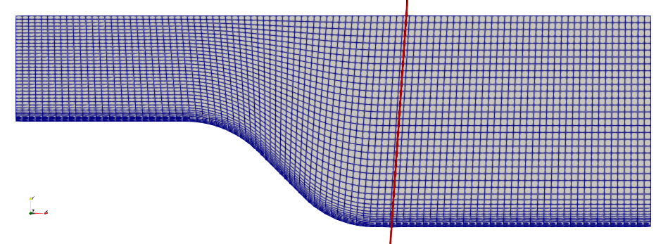
Fig. 1 Mesh and the vertical probe profile for a 45-degree ramp.
FIML for time-accurate unsteady flow over the ramp
To run this case, first download tutorials and untar it. Then go to tutorials-master/Ramp/unsteady/train and run the “preProcessing.sh” script.
./preProcessing.sh
Then, use the following command to run the case:
mpirun -np 4 python runScript.py 2>&1 | tee logOpt.txt
The setup is similar to the steady state FIML except that we consider both spatial and temporal evolutions of the flow. In other words, the trained model will improve both spatial and temporal predictions of the flow. We augment the SA model and make it match the k-omega SST model. Note: the default optimizer is SNOPT. If you don’t have access to SNOPT, you can also choose other optimizers, such as IPOPT and SLSQP.
Objective function: Regulated prediction error for the bottom wall pressure at all time steps
Design variables: Weights and biases for the built-in neural network
Augmented variables: betaFINuTilda for the nuTilda equations
Training configuration: U0 = 10 m/s
Prediction configuration: U0 = 5 m/s
The optimization exited with 50 iterations. The objective function reduced from 4.756E-01 to 3.274E-02.
Once the unsteady FIML is done. We can copy the last dict from designVariableHist.txt to tutorials-master/Ramp/unsteady/predict/trained. Then, go to tutorials-master/Ramp/unsteady/predict and run Allrun.sh. This command will run the primal for the baseline (SA), reference (k-omega SST), and the trained (FIML SA) models, similar to the steady-state case.
The following animation shows the comparison among these prediction case. The trained SA model significantly improves the spatial temporal evolution of velocity fields.
Fig. 2 Comparison among the reference, baseline, and trained models.
FIML for steady-state flow over the ramp (coupled FI and ML)
To run this case, first download tutorials and untar it. Then go to tutorials-master/Ramp/steady/train and run the “preProcessing.sh” script.
./preProcessing.sh
Then, use the following command to run the case:
mpirun -np 4 python runScript_FIML.py 2>&1 | tee logOpt.txt
This case uses our latest FIML interface, which incorporates a neural network model into the CFD solver to compute the augmented field variables (refer to the POF paper for details). We augment the k-omega model and make it match the k-omega SST model. The FIML optimization is formulated as:
Objective function: Regulated prediction error for the bottom wall pressure and the CD values
Design variables: Weights and biases for the built-in neural network
Augmented variables: betaFIK and betaFIOmega for the k and omega equations, respectively
Training configurations: c1: U0 = 10 m/s. c2: U0 = 20 m/s
Prediction configuration: U0 = 15 m/s
The optimization converged in 14 iterations, and the objective function reduced from 3.957E+01 to 3.542E+00.
To test the trained model’s accuracy for an unseen flow condition (i.e., U0 = 15 m/s), we can copy the designVariable.json (this file will be generated after the FIML optimization is done.) to tutorials-master/Ramp/steady/predict/trained. Then, go to tutorials-master/Ramp/steady/predict and run Allrun.sh. This command will run the primal for the baseline (k-omega), reference (k-omega SST), and the trained (FIML k-omega) models. The trained will read the optimized neural network weights and biases from designVariable.json, assign them to the built-in neural network model (defined in the regressionModel key in daOption) and run the primal solver.
For the U0 = 15 m/s case, the drag from the reference, baseline, and trained models are: 0.3881, 0.4458, 0.3829, respectively. The trained model significantly improve the drag prediction accuracy for this case.
FIML for steady-state flow over the ramp (decoupled FI and ML)
We can also first conduct field inversion, save the augmented fields and features to the disk, then conduct an offline ML to train the relationship between the features and augmented fields. This decoupled FIML approach was used in most of previous steady-state FIML studies.
First, generate the mesh and data for the c1 and c2 cases:
./preProcessing.sh
Then, use the following command to run FI for case c1:
mpirun -np 4 python runScript_FI.py -index=0 2>&1 | tee logOpt1.txt
After that, use the following command to run FI for case c2:
mpirun -np 4 python runScript_FI.py -index=1 2>&1 | tee logOpt2.txt
Once the above two FI cases converge, reconstruct the data for the last optimization iteration (for example, the last optimization iteration for case c1 is 0.0015, the last optimization iteration for case c2 is 0.0016). Copy c1/0.0015 to tf_training/c1_data. Copy c2/0.0016 to tf_training/c2_data.
Then, go to tf_training and run TensorFlow training:
python trainModel.py
After the training is done, it will save the model’s coefficients in a “model” folder. Copy this “model” folder to the c1 and c2 folders.
Lastly, we can use the trained model for prediction. For example, you can go to the c1 folder and run:
mpirun -np 4 python runPrimal.py -augmented=True 2>&1 | tee logOpt1.txt
Likewise, go to the c2 folder and run:
mpirun -np 4 python runPrimal.py -augmented=True 2>&1 | tee logOpt2.txt
DAFoam will read the trained tensorflow model, compute flow features, use the trained tensorflow model to compute the augmented fields, and run the primal flow solutions. In addition to runPrimal, you can also do an optimization using the trained model.