Post-processing

Check opt_IPOPT.txt for optimization progress and use Paraview to visualize flow fields.

Edit me

Fig. 1. Pressure and shape evaluation during the optimization process

Check optimization output file opt_IPOPT.txt

Once optimization is done, first check “opt_IPOPT.txt” in tutorials-main/NACA0012_Airfoil/incompressible. “opt_IPOPT.txt” contains the variation of functions with respect to the optimization iteration:

iter    objective    inf_pr   inf_du lg(mu)  ||d||  lg(rg) alpha_du alpha_pr  ls
   0  2.0820236e-02 2.26e-08 8.55e-02   0.0 0.00e+00    -  0.00e+00 0.00e+00   0
   1  2.0521266e-02 3.20e-04 6.86e-02  -5.9 9.91e-03    -  9.71e-01 1.00e+00h  1
   2  1.9623489e-02 2.54e-03 2.73e-01  -3.5 2.17e-02    -  9.75e-01 1.00e+00h  1
   3  1.9314850e-02 8.73e-04 6.61e-03  -4.3 2.10e-02    -  1.00e+00 1.00e+00h  1
   4  1.9241231e-02 1.72e-04 3.71e-03  -5.8 2.80e-02    -  1.00e+00 1.00e+00h  1
   5  1.9231794e-02 6.45e-06 8.07e-04  -6.2 9.33e-03    -  1.00e+00 9.97e-01h  1
   6  1.9170888e-02 7.57e-05 3.15e-03  -7.2 8.75e-02    -  1.00e+00 1.00e+00h  1
   7  1.9133030e-02 1.68e-04 1.09e-02  -6.9 1.07e+00    -  1.00e+00 2.23e-01h  3
   8  1.8913613e-02 2.22e-04 1.26e-02  -7.5 8.09e-01    -  1.00e+00 5.00e-01h  2
   9  1.8691236e-02 2.76e-03 1.64e-02  -6.8 6.77e+00    -  1.00e+00 1.66e-01h  2
iter    objective    inf_pr   inf_du lg(mu)  ||d||  lg(rg) alpha_du alpha_pr  ls
  10  1.9355900e-02 2.63e-03 3.41e-02  -6.5 1.07e+00    -  1.00e+00 8.96e-01H  1
  11  1.9355900e-02 2.63e-03 1.21e-01  -6.6 8.43e-01    -  1.51e-02 1.00e+00h  1
  12  1.7524672e-02 6.56e-02 2.01e-01  -6.6 2.76e+02    -  5.47e-03 1.33e-03h  1
  13  1.7855004e-02 2.39e-03 8.60e-03  -6.1 4.63e-01    -  1.00e+00 1.00e+00h  1
  14  1.7799861e-02 9.25e-04 3.58e-03  -7.0 2.62e-01    -  1.00e+00 1.00e+00h  1
  15  1.7800851e-02 1.32e-04 2.68e-03  -8.6 2.46e-01    -  1.00e+00 1.00e+00h  1
  16  1.7802465e-02 8.81e-06 6.38e-04  -7.5 2.70e-02    -  1.00e+00 1.00e+00h  1
  17  1.7802033e-02 2.50e-06 6.62e-05  -9.4 1.01e-02    -  1.00e+00 1.00e+00h  1
  18  1.7802058e-02 5.87e-09 2.90e-06 -11.0 1.17e-03    -  1.00e+00 1.00e+00h  1

The objective (CD) is 0.02082 for the baseline design and drops to 0.01780 for the 18th optimization iteration with a drag reduction of 14.5%. The optimality (inf_du) and feasibility (inf_pr) decrease to less than 1e-5.

Visualize the flow fields using Paraview

Next, we can use Paraview to visualize the flow fields. Download the Paraview binaries from here. They are ready to use for Windows, Linux, and MacOS. Once installed, open the Paraview app and click “File->Open…” from the top menu. In the pop-up window, navigate to tutorials-main/NACA0012_Airfoil/incompressible, select the paraview.foam file, and click “OK”.

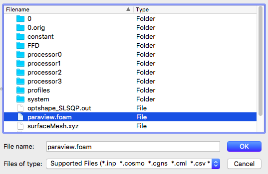
Note: paraview.foam is just a dummy file to tell ParaView where the case is located. paraview.foam itself does not contain any optimization data.

Fig. 2. Open the paraview.foam file

Then at the left panel, select “Decomposed Case” for “Case Type”.

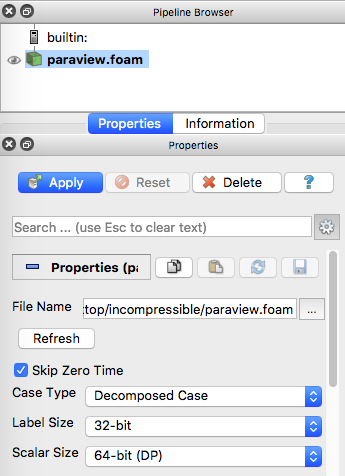
Note: The Decomposed Case type tells Paraview to load data from processor* folders since we ran this case in parallel using 4 CPU cores. If one runs a serial run with one CPU core, or you have reconstructed the intermediate result using the reconstructPar command, select Reconstructed Case.

Fig. 3. Select Case Type

Next, scroll down at the left panel and check “Camera Parallel Projection”.

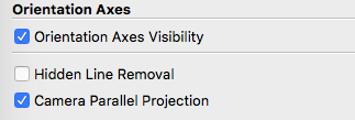
Note: The Camera Parallel Projection option is preferable for zoom-in visualization.

Fig. 4. Check Camera Parallel Projection

Now, click “Apply” at the left panel to load the flow fields. By default, the pressure field (p) will be load, but you can choose other flow variables to load at the top panel. Also, the “Surface” representation will be used by default, you can change it to “Surface With Edges” to visualize the mesh.

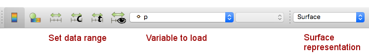
Fig. 5. Change variable to load and surface representation

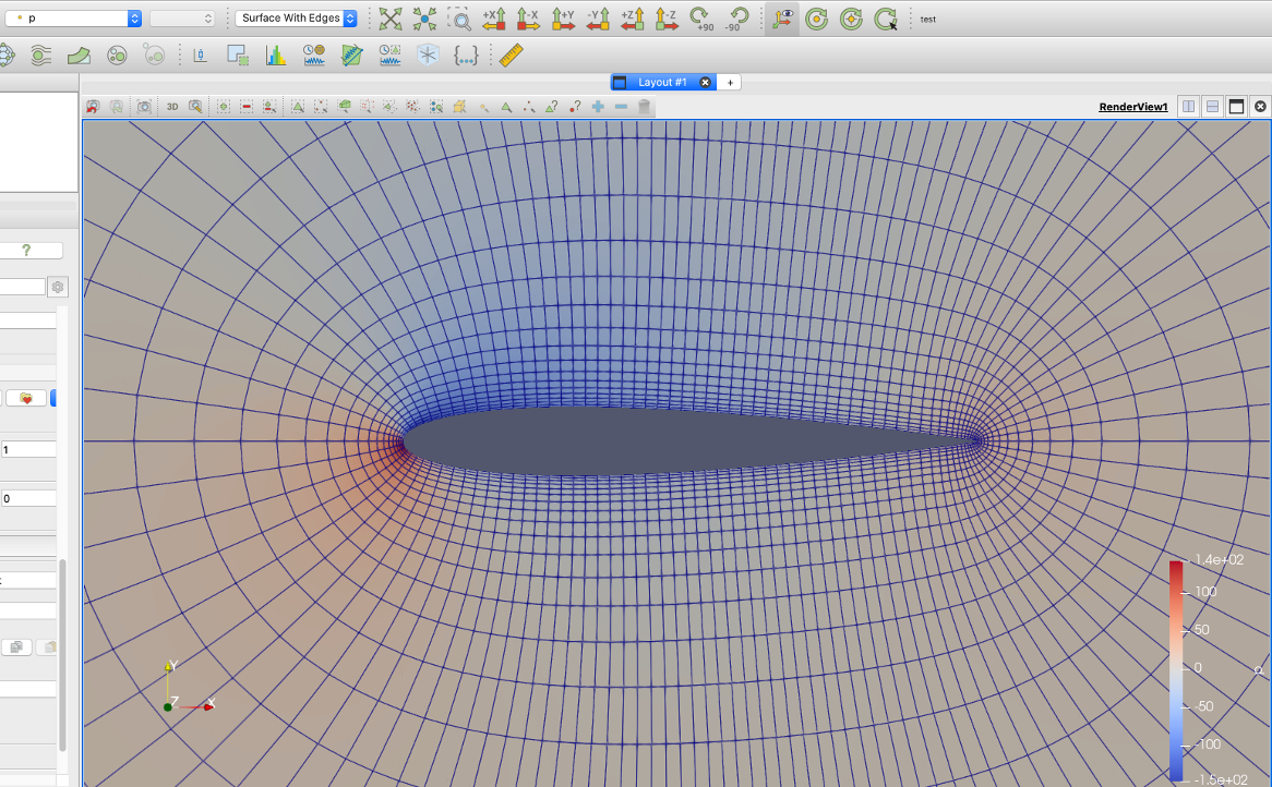
Fig. 6. Pressure contour and mesh for the NACA0012 case

Finally, you can hit the play button at the top panel to play a movie of the evolution of the pressure field and shape during the optimization (see the movie at the beginning of this page).

Fig. 7. Hit play to visualize a movie of the optimization process

Plot the surface pressure distribution using Paraview

To plot the surface pressure profile, you need to first click the “paraview.foam” from the “Pipeline Browser” window on the left. Then, unselect “internalMesh” and select “wing” in the “Mesh Regions” window on the left panel. After that, hit “Apply” to show the wing surface only. NOTE: By default, you will not “see” the wing surface because you are viewing from the z direction. You need to left click and drag to rotate the view.

Then, on the top menu, click “Sources-Search..” and search for the keyword “slice” and select it. Then on the left panel, click “Z Normal” and click “Apply” to cut a z-normal slice for the wing surface.

Then, right click “Slice1” from the “Pipeline Browser” and select “Add Filter-Data Analysis-Plot On Sorted Lines”, and then click “Apply”.

After that, you should see the plot on the right. By default, the plot is not for a pressure profile. You need to go to the left properties panel and choose “Points_X” for “X Array Name”, and then in the “Select Parameters” window, select “p” and unselect all other variables. NOTE: make sure you click the plot on the right to see its properties panel.

To save the raw data for the pressure profile, you can select the plotOnSortedLine1 on the left, and then click “Save Data” under the “File” menu.

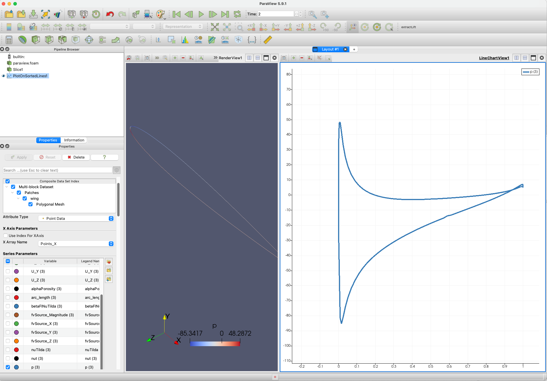
Fig. 7. Surface pressure distribution for the NACA0012 airfoil

Refer to the Paraview User Guide for more advanced usage.

In the next page, we will elaborate on optimization run scripts and configuration files.