This chapter was written by Zilong Li and reviewed by Ping He.
Learning Objectives:
After reading this chapter, you should be able to:
- Run the coupled and decoupled field inversion (FI) machine learning (ML) for steady-state and time-resolved unsteady flow problems
- Extend the FIML for new cases.
Overview
This tutorial elaborates on our latest field inversion machine learning (FIML) capability for steady-state and time-resolved unsteady flow problems. For more details, please refer to our POF paper.
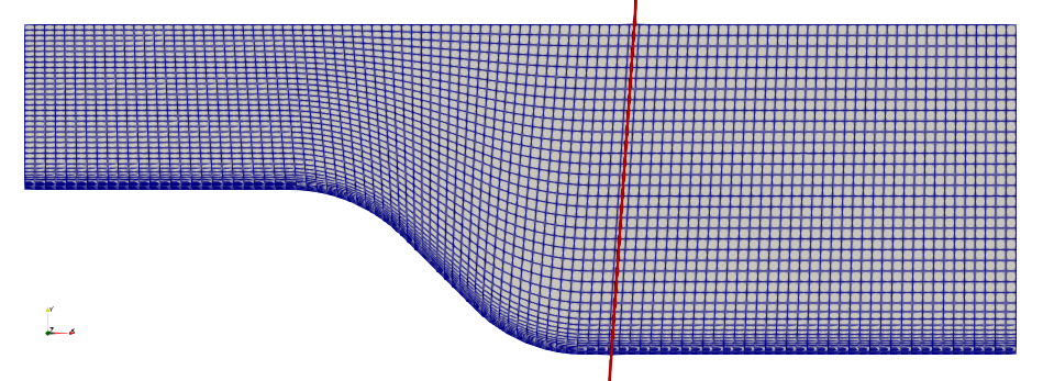
Fig. 1 Mesh and the vertical probe profile for a 45-degree ramp.
FIML for steady-state flow over the ramp (coupled FI and ML)
To run this case, first download tutorials and untar it. Then go to tutorials-master/Ramp/steady/train and run the “preProcessing.sh” script.
./preProcessing.sh
Before we run the case, let us elaborate on the runScript.py. We set the seed for NumPy’s random number generator to the integer value 1 so that we can obtain the exact same random results for every run. We have two training cases c1 and c2 (cases = [“c1”, “c2”]), and with the initial velocities 10 m/s and 20 m/s (U0s = [10.0, 20.0]), respectively. We also obtained the reference values for the drag (dragRefs = [0.1683, 0.7101]), their values can be obtained when we run the k-omega SST model. We also need to read the coordinates of the probe points from probePointCoords.json, which will be used by “UProbeVar” in the function component.
# =============================================================================
# Input Parameters
# =============================================================================

np.random.seed(1)

cases = ["c1", "c2"]
U0 = [10, 20.0]
CDData = np.array([0.1683, 0.7101])

with open("./probePointCoords.json") as f:
    probePointCoords = json.load(f)
In the “regressionModel” component, we need to set “active”: True when we run the regression model. We have two models: model1 and model2, basically they are almost the same, except in model1 our design variable (beta) is in the k equation, while in model2 the design variable is in the omega equation. We set “modelType”: “neuralNetwork”, which indicates that we use the neural network model. The inputs for the neural network model are four flow features: “PoD” (production / destruction), “Vos” (vorticity / strain), “PSoSS” (pressure normal stress / shear stress), and “KoU2” (turbulence intensity / velocity square). The neural network model has two hidden layers, and each has 20 neurons (“hiddenLayerNeurons”: [20, 20]). The four flow features have no input shift (“inputShift”: [0.0, 0.0, 0.0, 0.0]), and they are all scaled to 1 (“inputScale”: [1.0, 1.0, 1.0, 1.0]). We set both the outputShift and outputScale to 1 for the beta fields. And we select the “tanh” activation function for our neural network model. We set “writeFeatures”: True, so we will write the flow features to the disk.
    "regressionModel": {
        "active": True,
        "model1": {
            "modelType": "neuralNetwork",
            "inputNames": ["PoD", "VoS", "PSoSS", "KoU2"],
            "outputName": "betaFIK",
            "hiddenLayerNeurons": [20, 20],
            "inputShift": [0.0, 0.0, 0.0, 0.0],
            "inputScale": [1.0, 1.0, 1.0, 1.0],
            "outputShift": 1.0,
            "outputScale": 1.0,
            "activationFunction": "tanh",
            "printInputInfo": True,
            "defaultOutputValue": 1.0,
            "outputUpperBound": 1e1,
            "outputLowerBound": -1e1,
            "writeFeatures": True,
        },
        "model2": {
            "modelType": "neuralNetwork",
            "inputNames": ["PoD", "VoS", "PSoSS", "KoU2"],
            "outputName": "betaFIOmega",
            "hiddenLayerNeurons": [20, 20],
            "inputShift": [0.0, 0.0, 0.0, 0.0],
            "inputScale": [1.0, 1.0, 1.0, 1.0],
            "outputShift": 1.0,
            "outputScale": 1.0,
            "activationFunction": "tanh",
            "printInputInfo": True,
            "defaultOutputValue": 1.0,
            "outputUpperBound": 1e1,
            "outputLowerBound": -1e1,
            "writeFeatures": True,
        },
    },
Now let us elaborate on each entry in the function component.
        "pVar": {
            "type": "variance", # computes the variance of pressure between the original model and reference
            "source": "patchToFace",
            "patches": ["bot"], # extract from patch faces (patchToFace) on bottom patch ("bot")
            "scale": 1.0, # no scaling
            "mode": "surface", # surface variable
            "varName": "p",
            "varType": "scalar", # pressure is a scalar
            "timeDependentRefData": False, # not time dependent
        },
        "UFieldVar": {
            "type": "variance", # computes the variance of velocity field between the original model and reference
            "source": "boxToCell",
            "min": [-10.0, -10.0, -10.0],
            "max": [10.0, 10.0, 10.0], # extracted the velocity from all cells inside a bounding box (min and max define coordinates).
            "scale": 0.1, # scale down
            "mode": "field", # field variable
            "varName": "U",
            "varType": "vector", # veolicty is a vector
            "indices": [0, 1], # only x and y velocity components are considered
            "timeDependentRefData": False, # not time dependent
        },
        "UProbeVar": {
            "type": "variance", # computes the variance of velocity field at specific probe points between the original model and reference
            "source": "allCells",
            "scale": 1.0, # no scaling
            "mode": "probePoint",
            "probePointCoords": probePointCoords["probePointCoords"], # extract velocity at specific probe points (probePointCoords.json)
            "varName": "U",
            "varType": "vector", # veolicty is a vector
            "indices": [0, 1],  # only x and y velocity components are considered
            "timeDependentRefData": False, # not time dependent
        },
        "CDError": {
            "type": "force",
            "source": "patchToFace",
            "patches": ["bot"], # extract drag force from bottom patch
            "directionMode": "fixedDirection",
            "direction": [1.0, 0.0, 0.0], # drag direction is in the x-direction
            "scale": 1.0, # no scaling
            "calcRefVar": True, #computes the variance of drag force between the original model and reference
            "ref": [0.0],  # we will assign this later because each case has a different ref
        },
        "betaKVar": {
            "type": "variance",
            "source": "allCells",
            "scale": 0.01, # scale down
            "mode": "field", # field variable
            "varName": "betaFIK",
            "varType": "scalar", # betaFIK is a scalar
            "timeDependentRefData": False, # not time dependent
        },
        "betaOmegaVar": {
            "type": "variance",
            "source": "allCells",
            "scale": 0.01, # scale down
            "mode": "field", # field variable
            "varName": "betaFIOmega",
            "varType": "scalar", # betaFIOmega is a scalar
            "timeDependentRefData": False, # not time dependent
        },
Then, use the following command to run the case:
mpirun -np 4 python runScript.py 2>&1 | tee logOpt.txt
This case uses our latest FIML interface, which incorporates a neural network model into the CFD solver to compute the augmented field variables (refer to the POF paper for details). We augment the k-omega model and make it match the k-omega SST model. The FIML optimization is formulated as:
Objective function: Regulated prediction error for the bottom wall pressure and the CD values
Design variables: Weights and biases for the built-in neural network
Augmented variables: betaFIK and betaFIOmega for the k and omega equations, respectively
Training configurations: c1: U0 = 10 m/s. c2: U0 = 20 m/s
Prediction configuration: U0 = 15 m/s
The optimization converged in 14 iterations, and the objective function reduced from 3.957E+01 to 3.542E+00.
To test the trained model’s accuracy for an unseen flow condition (i.e., U0 = 15 m/s), we can copy the designVariable.json (this file will be generated after the FIML optimization is done.) to tutorials-master/Ramp/steady/predict/trained. Then, go to tutorials-master/Ramp/steady/predict and run Allrun.sh. This command will run the primal for the baseline (k-omega), reference (k-omega SST), and the trained (FIML k-omega) models. The trained will read the optimized neural network weights and biases from designVariable.json, assign them to the built-in neural network model (defined in the regressionModel key in daOption) and run the primal solver.
For the U0 = 15 m/s case, the drag from the reference, baseline, and trained models are: 0.3881, 0.4458, 0.3829, respectively. The trained model significantly improve the drag prediction accuracy for this case.
FIML for steady-state flow over the ramp (decoupled FI and ML)
We can also first conduct field inversion, save the augmented fields and features to the disk, then conduct an offline ML to train the relationship between the features and augmented fields. This decoupled FIML approach was used in most of previous steady-state FIML studies.
The decoupled FIML optimization is formulated as:
Objective function: Regulated prediction error for the bottom wall pressure, velocity at probe points and the CD values
Design variables: Weights and biases for the built-in neural network
Augmented variables: betaFIOmega for the omega equation
Training configurations: c1: U0 = 10 m/s. c2: U0 = 20 m/s
Prediction configuration: U0 = 15 m/s
First, generate the mesh and data for the c1 and c2 cases:
./preProcessing.sh
Before we run the case, let us elaborate on the runScript_FI.py, which is tailored for the decoupled FIML. The “idxI” is the input parameter that we use to get access to the cases, inital velocities U0s, and dragRefs (e.g, when we run the command mpirun -np 4 python runScript_FI.py -index=0 2>&1 | tee logOpt1.txt, the idxI will be set to 0). We have two training cases c1 and c2 (cases = [“c1”, “c2”]), and with the initial velocities 10 m/s and 20 m/s (U0s = [10.0, 20.0]), respectively. We also obtained the reference values for the drag (dragRefs = [0.1683459472347049, 0.7101215345814689]), their values can be obtained when we run the k-omega SST model. The parameter nCells is the number of cells for the mesh.
# =============================================================================
# Input Parameters
# =============================================================================

idxI = args.index
cases = ["c1", "c2"]
U0s = [10.0, 20.0]
dragRefs = [0.1683459472347049, 0.7101215345814689]
dragRef = dragRefs[idxI]
U0 = U0s[idxI]
case = cases[idxI]
nCells = 5000
In order to save the flow features, we need to set “outputName”: “dummy” (dummy means the neuralNetwork model will not be executed and only extract flow features) and “writeFeatures”: True in the “model”. In this case, we extract four flow features: “PoD” (production / destruction), “Vos” (vorticity / strain), “PSoSS” (pressure normal stress / shear stress), and “KoU2” (turbulence intensity / velocity square). We also have other flow features, for a exhaustive reference, you can refer to the file DARegression.C in the source code: “dafoam/src/adjoint/DARegression/DARegression.C”.
        "model": {
            "modelType": "neuralNetwork",
            "inputNames": ["PoD", "VoS", "PSoSS", "KoU2"],
            "outputName": "dummy",
            "hiddenLayerNeurons": [20, 20],
            "inputShift": [0.0, 0.0, 0.0, 0.0],
            "inputScale": [1.0, 1.0, 1.0, 1.0],
            "outputShift": 1.0,
            "outputScale": 1.0,
            "activationFunction": "tanh",
            "printInputInfo": True,
            "defaultOutputValue": 1.0,
            "outputUpperBound": 1e1,
            "outputLowerBound": -1e1,
            "writeFeatures": True,
        }
The following is the input setup for our design variable (beta), the “type” of beta is “field”, the “fieldName” of beta is “betaFIOmega” (when we want to augment the SA model, “betaFINutilda” should be choosen), the “fieldType” of beta is “scalar”, and we treat beta as a global field variable, so we set “distributed”: False, and the “components” key indicates that beta connect to the solver and function components.
    "inputInfo": {
        "beta": {
            "type": "field",
            "fieldName": "betaFIOmega",
            "fieldType": "scalar",
            "distributed": False,
            "components": ["solver", "function"],
        },
    },
In the configure(self) function, we need to add the design variables (beta) to the outout component, define the design variables to the top level, add the objective and connect any function in daOption to obj’s terms.
    def configure(self):
        # add the design variables to the dvs component's output
        self.dvs.add_output("beta", val=np.ones(nCells), distributed=False)
        self.connect("beta", "scenario1.beta")

        # define the design variables to the top level
        self.add_design_var("beta", lower=-5.0, upper=10.0, scaler=1.0)

        # add objective and constraints to the top level
        # we can connect any function in daOption to obj's terms
        self.connect("scenario1.aero_post.UFieldVar", "obj.error1")
        self.connect("scenario1.aero_post.dragVar", "obj.error2")
        self.connect("scenario1.aero_post.betaVar", "obj.regulation")
        self.add_objective("obj.val", scaler=1.0)
Then, use the following command to run FI for case c1:
mpirun -np 4 python runScript_FI.py -index=0 2>&1 | tee logOpt1.txt
After that, use the following command to run FI for case c2:
mpirun -np 4 python runScript_FI.py -index=1 2>&1 | tee logOpt2.txt
Once the above two FI cases converge, reconstruct the data for the last optimization iteration (for example, the last optimization iteration for case c1 is 0.0015, the last optimization iteration for case c2 is 0.0016). Copy c1/0.0015 to tf_training/c1_data. Copy c2/0.0016 to tf_training/c2_data.
Then, go to tf_training and run TensorFlow training:
python trainModel.py
After the training is done, it will save the model’s coefficients in a “model” folder. Copy this “model” folder to the c1 and c2 folders.
Lastly, we can use the trained model for prediction. For example, you can go to the c1 folder and run:
mpirun -np 4 python runPrimal.py -augmented=True 2>&1 | tee logOpt1.txt
Likewise, go to the c2 folder and run:
mpirun -np 4 python runPrimal.py -augmented=True 2>&1 | tee logOpt2.txt
DAFoam will read the trained tensorflow model, compute flow features, use the trained tensorflow model to compute the augmented fields, and run the primal flow solutions. In addition to runPrimal, you can also do an optimization using the trained model.
FIML for time-accurate unsteady flow over the ramp
To run this case, first download tutorials and untar it. Then go to tutorials-master/Ramp/unsteady/train and run the “preProcessing.sh” script.
./preProcessing.sh
Then, use the following command to run the case:
mpirun -np 4 python runScript.py 2>&1 | tee logOpt.txt
The setup is similar to the steady state FIML except that we consider both spatial and temporal evolutions of the flow. In other words, the trained model will improve both spatial and temporal predictions of the flow. We augment the SA model and make it match the k-omega SST model. Note: the default optimizer is SNOPT. If you don’t have access to SNOPT, you can also choose other optimizers, such as IPOPT and SLSQP.
Objective function: Regulated prediction error for the bottom wall pressure at all time steps
Design variables: Weights and biases for the built-in neural network
Augmented variables: betaFINuTilda for the nuTilda equations
Training configuration: U0 = 10 m/s
Prediction configuration: U0 = 5 m/s
The optimization exited with 50 iterations. The objective function reduced from 4.756E-01 to 3.274E-02.
Once the unsteady FIML is done. We can copy the last dict from designVariableHist.txt to tutorials-master/Ramp/unsteady/predict/trained. Then, go to tutorials-master/Ramp/unsteady/predict and run Allrun.sh. This command will run the primal for the baseline (SA), reference (k-omega SST), and the trained (FIML SA) models, similar to the steady-state case.
The following animation shows the comparison among these prediction case. The trained SA model significantly improves the spatial temporal evolution of velocity fields.
Fig. 2 Comparison among the reference, baseline, and trained models.
Questions
Run a decouple FI and ML steady case for a 2D NACA0012 airfoil:.
- Augment the SA model to match the results of k-omega SST model
- The Re = 1e6, the inlect velocity U = 10 m/s
- The angle of attack (AoA) for the airfoil is 12 degree
- Generate a mesh with ~10k cells
- Using the Cl from the k-omega SST model as the reference value
After the case is done:
- Compare the Cd and Cl differences between the baseline and reference, and the trained models and reference.
- Plot the Cp for the baseline, reference, and trained model.