OpenFOAM configurations
As mentioned in Overview, DAFoam uses OpenFOAM for multiphysics analysis. So, before running DAFoam optimizations, one needs to set up an OpenFOAM run case for the NACA0012 airfoil. tutorials-main/NACA0012_Airfoil/incompressible has the following folder structure:
NACA0012_Airfoil/incompressible
|-- 0.orig            # initial fields and boundary conditions (OpenFOAM essentials)
|-- FFD               # generate the FFD points
|-- constant          # flow and turbulence property definition (OpenFOAM essentials)
|-- profiles          # NACA0012 profile coordinate for mesh generation
|-- system            # flow discretization, setup, time step, etc (OpenFOAM essentials)
|-- Allclean.sh       # script to clean up the simulation and optimization results
|-- preProcessing.sh  # generate mesh, copy the initial and boundary conditions to 0
|-- genAirFoilMesh.py # mesh generation script called by preProcessing.sh
|-- paraview.foam     # dummy file for paraview post-processing
|-- runScript.py      # main run script for DAFoam
Here we assume you are familiar with the OpenFOAM setup. Otherwise, refer to the OpenFOAM tutorial guide for setting up the configuration files (i.e., the files in the 0, constant, and system folders).
preProcessing.sh
Once the OpenFOAM configuration files are properly set, we run the preProcessing.sh script to generate the mesh. This script first runs the genAirFoilMesh.py script to generate a hyperbolic mesh using pyHyp, saves the mesh to the plot3D format (volumeMesh.xyz).
Then it uses the OpenFOAM’s built-in utility plot3dToFoam to convert the plot3D mesh to the OpenFOAM mesh and save it to constant/polyMesh (plot3dToFoam -noBlank volumeMesh.xyz).
Since the plot3D mesh does not have boundary information, the converted OpenFOAM mesh has only one boundary patch, so we need to use the autoPatch utility to split boundaries (autoPatch 30 -overwrite). Here, 30 is the feature angle between two surface mesh faces. The utility will split patches if the feature angle is larger than 30 degrees.
The above split patches will have names such as auto0, auto1, auto2, we need to rename them to wing, sym, inout, etc. This is done by running createPatch -overwrite. The definition of boundary name is in system/createPatchDict.
Next, we call renumberMesh -overwrite to renumber the mesh points to reduce the bandwidth of Jacobians and reduce the memory usage. Finally, we copy the boundary condition files 0.orig to 0.
#!/bin/bash

# Check if the OpenFOAM environments are loaded
if [ -z "$WM_PROJECT" ]; then
  echo "OpenFOAM environment not found, forgot to source the OpenFOAM bashrc?"
  exit
fi

# generate mesh
echo "Generating mesh.."
python genAirFoilMesh.py &> logMeshGeneration.txt
plot3dToFoam -noBlank volumeMesh.xyz >> logMeshGeneration.txt
autoPatch 30 -overwrite >> logMeshGeneration.txt
createPatch -overwrite >> logMeshGeneration.txt
renumberMesh -overwrite >> logMeshGeneration.txt
echo "Generating mesh.. Done!"

# copy initial and boundary condition files
cp -r 0.orig 0
runScript.py
Once the OpenFOAM mesh is generated, we run mpirun -np 4 python runScript.py 2>&1 | tee logOpt.txt for optimization and save the detailed progress of optimization to logOpt.txt.
We first elaborate on the runScript.py script, which contains configurations for primal, adjoint, and optimization solutions.
The first section imports modules for DAFoam.
# =============================================================================
# Imports
# =============================================================================
import os
import argparse
import numpy as np
from mpi4py import MPI
import openmdao.api as om
from mphys.multipoint import Multipoint
from dafoam.mphys import DAFoamBuilder, OptFuncs
from mphys.scenario_aerodynamic import ScenarioAerodynamic
from pygeo.mphys import OM_DVGEOCOMP
from pygeo import geo_utils
In the next section, we define the optimizer to use in “-optimizer”. We use pyOptSparse to set optimization problems. pyOptSparse supports multiple open-source and commercial optimizers. However, in runScript.py, we only provide optimizer setup for IPOPT (default), SLSQP, and SNOPT. Refer to pyOptSparse documentation for all supported optimizers.
The “-task” argument defines the task to run, which includes “run_driver”: run optimization, “run_model”: run the primal analysis, “compute_totals”: run the adjoint derivative computation, “check_totals”: verify the adjoint accuracy against the finite-difference method.
We then define some global parameters such at “U0”: the far field velocity, “p0”: the far field pressure, “nuTilda0”: the far field turbulence variables, “CL_target”: the target lift coefficient, “alpha0”: the initial angle of attack, “A0” and “rho0”: the reference area and density to normalize drag and lift coefficients.
parser = argparse.ArgumentParser()
# which optimizer to use. Options are: IPOPT (default), SLSQP, and SNOPT
parser.add_argument("-optimizer", help="optimizer to use", type=str, default="IPOPT")
# which task to run. Options are: run_driver (default), run_model, compute_totals, check_totals
parser.add_argument("-task", help="type of run to do", type=str, default="run_driver")
args = parser.parse_args()

# =============================================================================
# Input Parameters
# =============================================================================
U0 = 10.0
p0 = 0.0
nuTilda0 = 4.5e-5
CL_target = 0.5
aoa0 = 5.13918623195176
A0 = 0.1
# rho is used for normalizing CD and CL
rho0 = 1.0
Next, the “daOptions” dictionary contains all the DAFoam parameters for primal and adjoint solvers. For a full list of input parameters in daOptions, refer to here.
“designSurfaces” is a list of patch names for the design surface to change during optimization. Here, “wing” is a patch in constant/polyMesh/boundary, and it needs to be of wall type.
“DASimpleFoam” is an incompressible solver that uses the SIMPLE algorithm, and it is derived from OpenFOAM’s built-in solver simpleFoam with modifications to compute adjoint derivatives.
The “primalMinResTol” parameter is the residual convergence tolerance for the primal solver (DASimpleFoam).
The “primalBC” dictionary defines the boundary conditions for the primal solution. Note that if primalBC is defined, it will overwrite the values defined in the 0 folder. Here we need to provide the variable name, patch names, and value to set for each variable. If “primalBC” is left blank, we will use the BCs defined in the 0 folder.
The “function” dictionary defines the objective and/or constraint functions. Taking “CD” as an example, we need to give a name to the function, e.g., “CD” or any other preferred name. We need to define the type of objective (e.g., “force”, “moment”; we need to use the reserved type names), how to select the discrete mesh faces to compute the objective (e.g., we select them from the name of a patch “patchToFace”), and the name of the patch (wing) for “patchToFace”. Since it is a force objective, we need to project the force vector to a specific direction. Here, we define “CD” as the force that is parallel to the flow direction (“parallelToFlow”). Alternative, we can also use “fixedDirection” and provide a “direction” key for force, i.e., “directionMode”: “fixedDirection”, “direction”: [1.0, 0.0, 0.0]. Since we select “parallelToFlow”, we need to prescribe the name of the patch for velocity input (“patchV”) design variable to determine the flow direction. NOTE: if no “patchV” is defined in inputInfo, we can NOT use “parallelToFlow”. For this case, we have to use “directionMode”: “fixedDirection” instead. The “scale” parameter is a scaling factor for this objective “CD”, i.e., CD = force / (0.5 * U0 * U0 * A0 * rho0). The definition of “CL” is similar to “CD” except that we use “normalToFlow” for “directionMode”.
The “adjEqnOption” dictionary contains the adjoint linear equation solution options. If the adjoint does not converge, increase “pcFillLevel” to 2. Or try “jacMatReOrdering” : “nd”. By default, we require the adjoint equation to drop six orders of magnitude.
“normalizeStates” contains the state normalization values. Here, we use the far-field values as a reference. NOTE: Since “p” is relative, we use the dynamic pressure “U0 * U0 / 2”. For compressible flow, we can just use p0. Also, the face flux variable phi will be automatically normalized by its surface area, so we can set “phi”: 1.0. We also need to normalize the turbulence variables, such as nuTilda, k, omega, and epsilon.
Finally, we define the input variables in the “inputInfo” dictionary. “inputInfo” defines the input variables for a component in OpenMDAO. Each key in “inputInfo” defines an input variable for a component, specified by the “components” key. One input can also be connected to multiple components. The name of the key in “inputInfo” is the name of the input for that component. The “type” key defines the type of this input. Each input type has its own customized keys, such as “patches” for “patchVelocity” shown below.
daOptions = {
    "designSurfaces": ["wing"],
    "solverName": "DASimpleFoam",
    "primalMinResTol": 1.0e-8,
    "primalBC": {
        "U0": {"variable": "U", "patches": ["inout"], "value": [U0, 0.0, 0.0]},
        "p0": {"variable": "p", "patches": ["inout"], "value": [p0]},
        "nuTilda0": {"variable": "nuTilda", "patches": ["inout"], "value": [nuTilda0]},
        "useWallFunction": True,
    },
    "function": {
        "CD": {
            "type": "force",
            "source": "patchToFace",
            "patches": ["wing"],
            "directionMode": "parallelToFlow",
            "patchVelocityInputName": "patchV",
            "scale": 1.0 / (0.5 * U0 * U0 * A0 * rho0),
        },
        "CL": {
            "type": "force",
            "source": "patchToFace",
            "patches": ["wing"],
            "directionMode": "normalToFlow",
            "patchVelocityInputName": "patchV",
            "scale": 1.0 / (0.5 * U0 * U0 * A0 * rho0),
        },
    },
    "adjEqnOption": {"gmresRelTol": 1.0e-6, "pcFillLevel": 1, "jacMatReOrdering": "rcm"},
    "normalizeStates": {
        "U": U0,
        "p": U0 * U0 / 2.0,
        "nuTilda": nuTilda0 * 10.0,
        "phi": 1.0,
    },
    "inputInfo": {
        "aero_vol_coords": {"type": "volCoord", "components": ["solver", "function"]},
        "patchV": {
            "type": "patchVelocity",
            "patches": ["inout"],
            "flowAxis": "x",
            "normalAxis": "y",
            "components": ["solver", "function"],
        },
    },
}
Next, we need to define the mesh deformation option. Users need to manually provide the point and normal of all symmetry planes for “symmetryPlanes” in meshOptions.
# mesh warping parameters
meshOptions = {
    "gridFile": os.getcwd(),
    "fileType": "OpenFOAM",
    # point and normal for the symmetry plane
    "symmetryPlanes": [[[0.0, 0.0, 0.0], [0.0, 0.0, 1.0]], [[0.0, 0.0, 0.1], [0.0, 0.0, 1.0]]],
}
Next, we use the Mphys interface to set up the optimization problem. Mphys is based on OpenMDAO and allows us to develop multidisciplinary optimization capability in a modular way. If you are not familiar with OpenMDAO, check OpenMDAO documentation. We suggest you read the “Getting Started”, “Basic user guide”, and “Advanced user guide” (optional).
The following is the OpenMDAO N2 diagram that illustrates the inputs and outputs of components and their interaction in an optimization problem. The Top class will essentially create the components and set the proper connection.
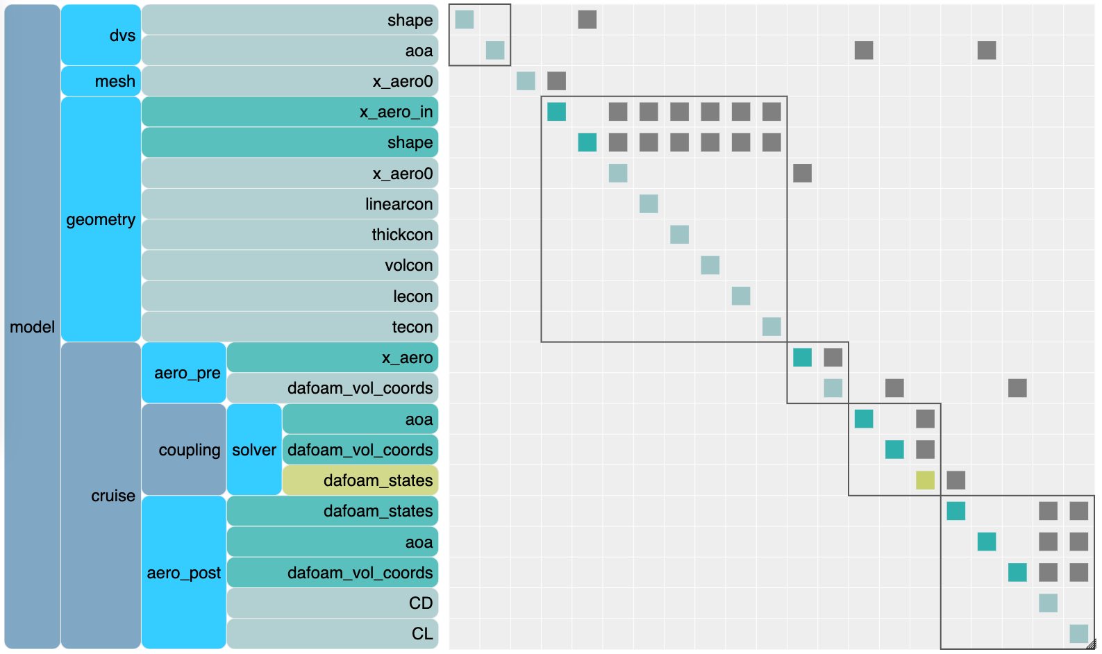
Fig. 1. The OpenMDAO N2 diagram for the airfoil aerodynamic optimization problem.
In the above diagram, blue is the groups, cyan is the components, light green is the outputs, and dark green is the inputs. The yellow denotes the outputs computed implicitly.
In the setup(self) function, we need to create all components for this problem. We first create the builder to initialize the DASolvers. This step will initialize the memory for all the variables in the OpenFOAM layer.
dafoam_builder = DAFoamBuilder(daOptions, meshOptions, scenario="aerodynamic")
dafoam_builder.initialize(self.comm)
Then, we call the self.add_subsystem interface to add components (dvs, mesh, geometry) for the optimization problem.
The dvs component is a special component that has only outputs. We usually use its outputs as the input variables (shape and patchV).
The mesh component has the airfoil surface mesh coordinates as the output. It is used as the initial design surface coordinates.
The geometry component is based on pyGeo. pyGeo uses the free-form deformation (FFD) approach to manipulate the design surface geometry. Here, pyGeo takes the baseline surface mesh and the shape variables as input and outputs the deformed surface mesh x_aero0, as well as all the geometry constraints (defined later in this script). The FFD point file (wingFFD.xyz) is loaded to the geometry (pyGeo) component. NOTE: The FFD volume should completely contain the design surface (see the red dots from this page). The FFD file wingFFD.xyz is generated by running “python genFFD.py” in the FFD folder.
We also add an aerodynamic scenario called “scenario1”. Refer to the above N2 diagram. We pass the dafoam_builder to the scenario1 scenario and allow it to manipulate the variables in the OpenFOAM layer to compute flow and derivatives.
In the scenario1 group, we have the aero_pre component, which is based on IDWarp. IDWarp uses an inverse-distance weighted algorithm to deform the volume mesh coordinates based on the surface mesh deformation, computed by pyGeo. Once the volume mesh is deformed, IDWarp outputs it as aero_vol_coords.
Then, the aero_vol_coords is passed to the solver component, along with the patchV from the dvs component. The solver (DAFoam) will compute the state variables aero_states.
Finally, the converged state aero_states, patchV, and aero_vol_coords will be passed to the aero_post component to compute the objective and constraint functions (CD and CL).
Note that we need to only setup the component and data transfer, and OpenMDAO will automatically compute the total derivatives using the adjoint method.
# add the design variable component to keep the top level design variables
self.add_subsystem("dvs", om.IndepVarComp(), promotes=["*"])

# add the mesh component
self.add_subsystem("mesh", dafoam_builder.get_mesh_coordinate_subsystem())

# add the geometry component (FFD)
self.add_subsystem("geometry", OM_DVGEOCOMP(file="FFD/wingFFD.xyz", type="ffd"))

# add a scenario (flow condition) for optimization, we pass the builder
# to the scenario to actually run the flow and adjoint
self.mphys_add_scenario("scenario1", ScenarioAerodynamic(aero_builder=dafoam_builder))
Next, we manually connect the surface mesh coordinates between the mesh, geometry, and scenario1 components.
# need to manually connect the x_aero0 between the mesh and geometry components
# here x_aero0 means the surface coordinates of structurally undeformed mesh
self.connect("mesh.x_aero0", "geometry.x_aero_in")
# need to manually connect the x_aero0 between the geometry component and the scenario1
# scenario group
self.connect("geometry.x_aero0", "scenario1.x_aero")
In the configure(self) function, we need to set up more details for each component (e.g., set the input and output). We add the surface coordinates to the geometry component, and we set the triangular points for geometric constraints.
# get the surface coordinates from the mesh component
points = self.mesh.mphys_get_surface_mesh()

# add pointset to the geometry component
self.geometry.nom_add_discipline_coords("aero", points)

# set the triangular points to the geometry component for geometric constraints
tri_points = self.mesh.mphys_get_triangulated_surface()
self.geometry.nom_setConstraintSurface(tri_points)
Next, we use the shape function to define shape variables for 2D airfoil. The symmetrical, leading edge (LE), and trailing edge (TE) constraints are also defined here. The symmetrical constraint is applied by making k=0 and k=1 move together. The LE/TE constraints are applied by making j=0 and j=1 move in opposite directions. The LE/TE constraints are needed because we do not want the shape variable to change the pitch and, therefore, the angle of attack. Instead, we want to change the far field velocity direction for the angle of attack.
# use the shape function to define shape variables for 2D airfoil
pts = self.geometry.DVGeo.getLocalIndex(0)
dir_y = np.array([0.0, 1.0, 0.0])
shapes = []
for i in range(1, pts.shape[0] - 1):
    for j in range(pts.shape[1]):
        # k=0 and k=1 move together to ensure symmetry
        shapes.append({pts[i, j, 0]: dir_y, pts[i, j, 1]: dir_y})
# LE/TE shape, the j=0 and j=1 move in opposite directions so that
# the LE/TE are fixed
for i in [0, pts.shape[0] - 1]:
    shapes.append({pts[i, 0, 0]: dir_y, pts[i, 0, 1]: dir_y, pts[i, 1, 0]: -dir_y, pts[i, 1, 1]: -dir_y})
self.geometry.nom_addShapeFunctionDV(dvName="shape", shapes=shapes)
Next, we setup the volume, thickness, and leading edge radius constraints.
We need to first define the leading (“leList”) and trailing (“teList”) edges. For example, the leList includes two points that defines a straight line that is parallel to the leading edge. The straight line in leList should be close to the leading edge and completely within the wing surface mesh.
To compute the volume, pyGeo first constructs a 2D mesh from the “leList” and “teList”. Here “nSpan = 2” and “nChord = 10” mean we use two points in the spanwise (z) and 10 points in the chordwise (x) to construct the 2D mesh. Then pyGeo projects this 2D mesh upward and downward to the wing surface mesh and forms 3D trapezoid volumes to approximate the wing volume. The more the leList and teList are close to the actual leading and trailing edges of the airfoil mesh, the better the volume approximation will be. Also, increasing the nSpan and nChord gives a better volume approximation. We recommend nSpan and nChord be similar to the number of FFD points in the spanwise and chordwise directions.
The thickness constraints are handled in a similar manner. Similar to the volume constraint, pyGeo first constructs a 2 by 10 mesh from the leList and teList and projects the 2D mesh points upward and downward to the wing surface to compute the thickness at these 20 locations; we have 20 thickness constraints in total.
For a more detailed explanation of constraint setup, refer to MACH-Aero-Tutorials.
# setup the volume and thickness constraints
leList = [[1e-4, 0.0, 1e-4], [1e-4, 0.0, 0.1 - 1e-4]]
teList = [[0.998 - 1e-4, 0.0, 1e-4], [0.998 - 1e-4, 0.0, 0.1 - 1e-4]]
self.geometry.nom_addThicknessConstraints2D("thickcon", leList, teList, nSpan=2, nChord=10)
self.geometry.nom_addVolumeConstraint("volcon", leList, teList, nSpan=2, nChord=10)
self.geometry.nom_addLERadiusConstraints("rcon", leList, 2, [0.0, 1.0, 0.0], [-1.0, 0.0, 0.0])
# NOTE: we no longer need to define the sym and LE/TE constraints
# because these constraints are defined in the above shape function
Next, we set the outputs for the dvs component and use them as the design (input) variables. We also need to connect the output of dvs component to the scenario1 and geometry components. Check the above N2.
# add the design variables to the dvs component's output
self.dvs.add_output("shape", val=np.array([0] * len(shapes)))
self.dvs.add_output("patchV", val=np.array([U0, aoa0]))
# manually connect the dvs output to the geometry and scenario1
self.connect("patchV", "scenario1.patchV")
self.connect("shape", "geometry.shape")
We then define the design variables to the top level, note that we fix the free-stream velocity U0 and allow aoa to change.
# define the design variables to the top level
self.add_design_var("shape", lower=-1.0, upper=1.0, scaler=10.0)
# here we fix the U0 magnitude and allows the aoa to change
self.add_design_var("patchV", lower=[U0, 0.0], upper=[U0, 10.0], scaler=0.1)
Finally, we setup the objective and constraint functions. Here we use relative upper and lower bound values with respect to the initial volume (default).
# add objective and constraints to the top level
self.add_objective("scenario1.aero_post.CD", scaler=1.0)
self.add_constraint("scenario1.aero_post.CL", equals=CL_target, scaler=1.0)
self.add_constraint("geometry.thickcon", lower=0.5, upper=3.0, scaler=1.0)
self.add_constraint("geometry.volcon", lower=1.0, scaler=1.0)
self.add_constraint("geometry.rcon", lower=0.8, scaler=1.0)
Once the Top class is defined, we pass it to the OpenMDAO problem and write a N2 diagram for this problem.
# OpenMDAO setup
prob = om.Problem()
prob.model = Top()
prob.setup(mode="rev")
om.n2(prob, show_browser=False, outfile="mphys.html")
The optimizer parameters are defined next. We use the pyOptSparse interface to optimizers.
# use pyoptsparse to setup optimization
prob.driver = om.pyOptSparseDriver()
prob.driver.options["optimizer"] = args.optimizer
# options for optimizers
if args.optimizer == "SNOPT":
    prob.driver.opt_settings = {
        "Major feasibility tolerance": 1.0e-5,
        "Major optimality tolerance": 1.0e-5,
        "Minor feasibility tolerance": 1.0e-5,
        "Verify level": -1,
        "Function precision": 1.0e-5,
        "Major iterations limit": 100,
        "Nonderivative linesearch": None,
        "Print file": "opt_SNOPT_print.txt",
        "Summary file": "opt_SNOPT_summary.txt",
    }
elif args.optimizer == "IPOPT":
    prob.driver.opt_settings = {
        "tol": 1.0e-5,
        "constr_viol_tol": 1.0e-5,
        "max_iter": 100,
        "print_level": 5,
        "output_file": "opt_IPOPT.txt",
        "mu_strategy": "adaptive",
        "limited_memory_max_history": 10,
        "nlp_scaling_method": "none",
        "alpha_for_y": "full",
        "recalc_y": "yes",
    }
elif args.optimizer == "SLSQP":
    prob.driver.opt_settings = {
        "ACC": 1.0e-5,
        "MAXIT": 100,
        "IFILE": "opt_SLSQP.txt",
    }
else:
    print("optimizer arg not valid!")
    exit(1)
Finally, we select the proper task to run. By default, the script will run findFeasibleDesign to find the correct aoa to get the target lift, and then start the optimization. You can also do runPrimal (solve the primal once), runAdjoint (run the primal and adjoint once), or checkTotals (compare the adjoint derivatives with the finite-difference references.)
if args.task == "run_driver":
    # solve CL
    optFuncs.findFeasibleDesign(["scenario1.aero_post.CL"], ["patchV"], targets=[CL_target], designVarsComp=[1])
    # run the optimization
    prob.run_driver()
elif args.task == "run_model":
    # just run the primal once
    prob.run_model()
elif args.task == "compute_totals":
    # just run the primal and adjoint once
    prob.run_model()
    totals = prob.compute_totals()
    if MPI.COMM_WORLD.rank == 0:
        print(totals)
elif args.task == "check_totals":
    # verify the total derivatives against the finite-difference
    prob.run_model()
    prob.check_totals(compact_print=False, step=1e-3, form="central", step_calc="abs")
else:
    print("task arg not found!")
    exit(1)
In the next section, we will elaborate on some common modifications for this case.