This chapter was written by Ping He.
Learning Objectives:
This chapter includes a very brief introduction to gradient-based optimization. For more detailed information, refer to Martins and Ning’s MDO book.
After reading this chapter, you should be able to:
- Explain the overall steps in a gradient-based design optimization.
- Identify and describe key terminology, including the objective function, design variables, constraints, and residuals.
Constrained gradient-based optimization
Optimization problem formulation
DAFoam solves constrained nonlinear optimization problems using gradient-based optimization algorithms, with the gradients efficiently computed by the discrete adjoint method. In such problems, an objective function $f(\vec{x})$ is minimized by changing the design variables ($\vec{x}$), subject to certain constraints $\vec{g}(\vec{x})$ and $\vec{h}(\vec{x})$.
\[\begin{aligned} \text{minimize: } & f(\vec{x}), \\ \text{with respect to: } & \vec{x} \\ \text{subject to: } & \vec{h}(\vec{x}) = 0, \\ & \vec{g}(\vec{x}) \le 0. \end{aligned}\]Here, $f$ is a scalar objective function to be minimized, and $\vec{x}$ is the vector of design variables, i.e., the variables we can modify in the design. $\vec{g}(\vec{x})$ and $\vec{h}(\vec{x})$ are the inequality and equality constraint functions, respectively. Here, we want to enforce $\vec{h}(\vec{x}) = 0$ and $\vec{g}(\vec{x}) \le 0$, thereby restricting the feasible design space. Note that $f$, $\vec{g}$, and $\vec{h}$ must be either explicit or implicit functions of the design variables $\vec{x}$. $f(\vec{x})$, $\vec{h}(\vec{x})$, and $\vec{g}(\vec{x})$ can be either linear or nonlinear functions. The inequality constraint is “active”, if $\vec{g}(\vec{x}) = 0$; otherwise, it is “inactive” if $\vec{g}(\vec{x}) \lt 0$. All equality constraints are active because we need $\vec{h}(\vec{x}) = 0$.
A typical example is airfoil aerodynamic shape optimization, where the objective function is the drag coefficient $C_d$, the design variables $\vec{x}$ are control points that change the airfoil shape, and the constraints include a lift (equality) constraint ($C_l=0.5$) and a moment (inequality) constraint $C_m \le b$. Here both the objective and constraint functions are implicit functions of the design variables.
Iterative optimization process
In general, the above optimization problem can not be solved analytically, so we need to use an iterative approach to find the optimal solution $\vec{x}$. The iterative optimization process starts with an initial guess of the design variables $\vec{x}_0$, called the initial design or baseline design. Then, an optimization algorithm computes a search direction and step size to update the design variable using
\[\vec{x}^{n+1} = \vec{x}^n + \alpha^n \vec{d}^n\]Here $n$ is the optimization iteration number, $\alpha$ is a scalar step size, and $\vec{d}$ is the search direction vector. $\vec{d}$ and $\vec{x}$ have the same size.
An example of iterative optimization processes for a 2D optimization problem is illustrated in the following figure. Here, the x and y axes are the two design variables, and the contour denotes the value of the objective function. The baseline design $\vec{x}^0$ is located in the bottom left region of the 2D design space. The next design variables are computed using $\vec{x}^1=\vec{x}^0+\alpha^0 \vec{d}^0$. This process is repeated until the optimal design point ($\vec{x}^*$) is found.
NOTE: During optimization, linear constraints will always be satisfied at each optimization iteration. However, nonlinear constraints may be violated in early iterations, and they will be eventually satisfied when the optimization converges.
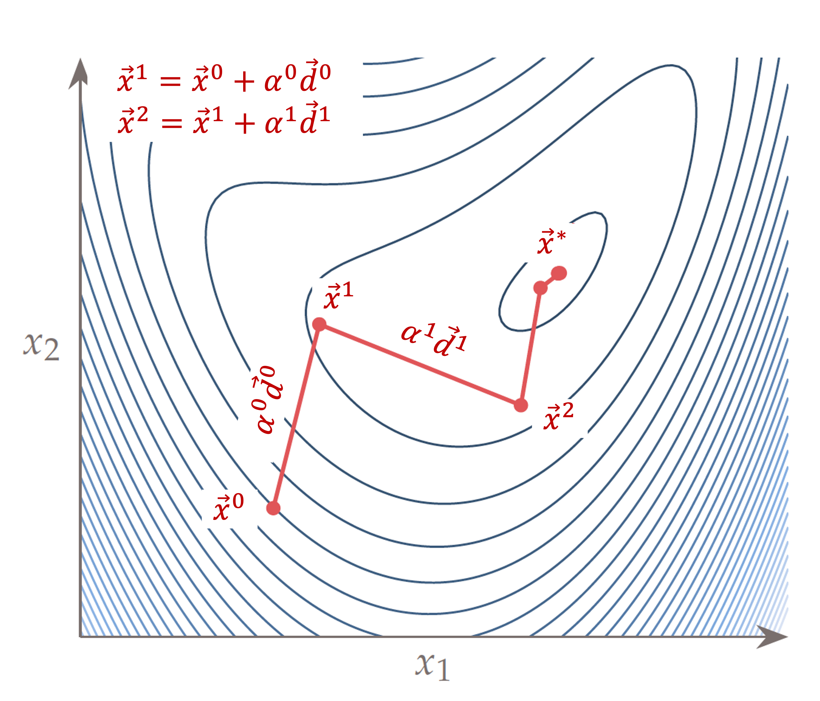
Fig. 1. Schematic of an iterative optimization process for a 2D problem
Objective function evaluation
For simple optimization problems, the objective function ($f$) is an explicit function of the design variable $\vec{x}$, so we can directly compute the $f$ value for a given set of $\vec{x}$ values. However, for many engineering design problems, the objective function ($f$) is an implicit function of the design variable $\vec{x}$. In this case, $f$ depends on both the state variables $\vec{w}$ and design variable $\vec{x}$, and they are correlated by a governing equation $\vec{R}(\vec{w}, \vec{x})=0$. The objective function evaluation consists of two steps (see the following figure). 1. Use $\vec{x}$ as the input to solve the governing equation and obtain the converged state variable $\vec{w}$. 2. Use $\vec{x}$ and $\vec{w}$ as the inputs to compute $f(\vec{w}, \vec{x})$. In design optimization, we call the step 1 the primal solution. One example is to solve the Navier-Stokes governing equation to get the state variables (flow fields), and then use the flow fields (state variables) to compute the drag coefficient (objective function). We will discuss the details of primal solutions later.
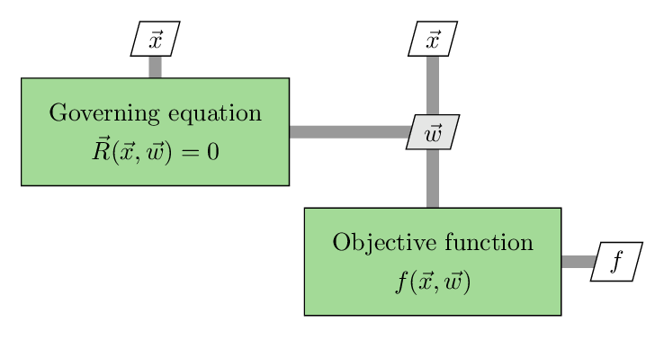
Fig. 2. Schematic of the objective function computation process
Search direction computation
The search direction $\vec{d}$ is typically computed based on the gradient vector $\nabla f = \text{d}f/\text{d}\vec{x}$. The gradient vector represents the sensitivity of the objective function with respect to the change in the design variable. Therefore, if the objective is very sensitive to a design variable $x_i$, i.e., $\text{d}f/\text{d}\vec{x}_i$ is large, the optimizer tends to change $x_i$ more than other design variables. In practice, we may need to manually scale the design variables (e.g., change the unit from m to mm) to control how we want the optimizer to make the change.
In the steepest descent optimization algorithm, the search direction is simply the opposite direction of the normalized gradient vector $\vec{d} = - \nabla f / \lvert \nabla f \rvert$. For more advanced optimization algorithms, such as sequential quadratic programming (SQP), the search direction is typically a complex function of the gradient vector. For large-scale optimization problems with hundreds of design variables, computing gradients becomes computationally expensive. So, DAFoam uses the discrete adjoint method to efficiently compute the gradients, which will be discussed later.
Step size computation (line search)
Once the search direction $\vec{d}$ is computed, we need to take a step size to actually update the design variable. The step size determination is always a 1D problem, no matter how many design variables we have. So, this process is also called line search. The process typically starts with trying a default step size to update the design, i.e., $\vec{x}^{n+1} = \vec{x}^n + \alpha^\textrm{init} \vec{d}^n$. Then, we can use this new candidate design variable to evaluate $f$ (call the primal solution). If the objective function $f$ is reduced (the design is improved for this iteration), we accept the step size. Otherwise, if $f$ increases instead of decreasing, or the new design is infeasible (e.g., negative mass or negative mesh volume), we may reduce the step size by a factor, e.g., 0.1, and compute a new candidate design variable vector. This line search process will be repeated until $f$ is reduced for this iteration. The line search ensures the objective function always reduces for all optimization iterations. Note that each line search iteration requires calling the primal solution once.
Convergence criteria
At the optimal point, the first-order necessary condition states that the gradients need to be zero. Therefore, many optimizers print out the optimality value, which measures the magnitude of the gradient vector. If an optimization converges well, we should see a decrease in the objective function during the optimization process, along with a decrease in the optimality. In theory, we also need to verify the second-order sufficient condition (a positive definitive Hessian) for an optimal point; however, this is often ignored since computing accurate Hessians can be expensive. For constrained optimization problems, we also require that all constraints are satisfied at the optimal point. This can be measured by the feasibility metric, which measures the violation of all constraints. If the feasibility is small, we consider the design point to be a feasible optimal point. Note that constrained optimization should start with a feasible, baseline design with at least one active constraint to ensure fair comparisons.
Primal simulation using numerical methods
Numerical methods and discretization
As mentioned above, we need to solve a set of governing equations, $\vec{R}(\vec{w}, \vec{x}) = 0$, to obtain the state variables and evaluate the objective function. This process is called the primal solution in the context of design optimization. For many engineering problems, such as those governed by the Navier–Stokes equations, analytical solutions are infeasible due to the complexity of the equations. To address this, we can use numerical methods that approximate the solution over a finite number of spatial (mesh) and temporal (time step) intervals, a process also known as discretization.
Taking the following figure as an example. We divide the simulation domain into smaller pieces, called mesh cells. Then, we solve for the state variables, such as velocity, pressure, and density, only for these discrete mesh cells. By doing this, the original continuous problems become discrete, and solving the states for these discrete mesh cells becomes computationally feasible. For example, we can approximate the first-order spatial derivative, defined in continuous space, by using the information from discrete space (mesh cells):
\[\frac{\partial u}{\partial x}_i = \frac{u_{i+1} - u_{i-1}}{2\Delta x}\]Here, the subscript i denotes the mesh cell index, and $\Delta x$ is the mesh size.
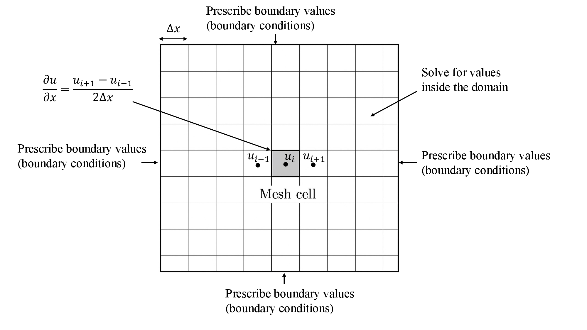
Fig. 3. A schematic of spatial discretization for a 2D simulation domain
Initial and boundary conditions
Although the above numerical analysis makes the solution of complex governing equations feasible, there are an infinite number of discrete solutions that satisfy the governing equations. To make the solution unique and relevant to the specific problem we are interested in, we need to prescribe proper initial and boundary conditions to the problem. The initial conditions are the initial values for all state variables, before the simulation starts. The boundary conditions are the state variable values at the outer boundary of the simulation domain. In general, we can set two types of boundary conditions: Dirichlet (fixed-value) and Neumann (fixed-gradient). Refer to the figure above.
Solution of the discretized governing equations
After discretizing the simulation domain and setting proper initial and boundary conditions, we will get a set of discretized governing equations. These equations can often be written as $\mathbf{A}\vec{w}=\vec{b}$, where $A$ is a matrix that contains all the discretization operators, $\vec{w}$ is the state variables (solutions), and $\vec{b}$ is the right-hand side (constant) operators from the discretization. For general nonlinear governing equations, both $A$ and $\vec{b}$ can be functions of the state variables $\vec{w}$ and design variables $\vec{x}$. Then, the primal solver will solve the above equation in an iterative manner (e.g., using the Gauss-Seidel method). To monitor the convergence, we often print out the residuals during the primal solution process. Here the primal residuals are defined as $\vec{R} = \mathbf{A}\vec{w} - \vec{b}$.
Gradient computation using the discrete adjoint method
DAFoam uses the discrete adjoint method to compute gradients efficiently. A key advantage of this approach is that its computational cost is independent of the number of design variables. Adjoint-based gradient computation involves two main steps:
1 Solving the adjoint equation
\[\frac{\partial \vec{R}}{\partial \vec{w}}^T \vec{\psi} = \frac{\partial f }{\partial \vec{w}}^T\]Here $\vec{\psi}$ is the adjoint vector, and the superscript $T$ denotes the transpose operator. The above adjoint equation is a large-scale linear equation, and DAFoam uses the generalized minimal residual method (GMRES) to solve it. During the GMRES solution processes, the adjoint residual measures the difference between the left and right-hand side of the above equation.
2 Computing the total derivative:
\[\frac{\text{d} f }{\text{d} \vec{x}} = \frac{\partial f }{\partial \vec{x}} - \frac{\partial \vec{R} }{\partial \vec{x}}^T \vec{\psi}\]In this step, the total derivative of the objective function with respect to the design variables $\vec{x}$ is computed explicitly, using the adjoint vector $\vec{\psi}$ computed from step 1. Since the design variables do not appear in the adjoint equation, only one adjoint solve per objective function is needed, regardless of the number of design variables. The second equation is non-iterative and computationally inexpensive. DAFoam computes all partial derivatives and matrix–vector products using automatic differentiation (AD) for accuracy and efficiency.
Questions
-
How to maximize the objective function?
-
How many primal and adjoint solutions are needed in one optimization iteration? Why?
-
Why do we need to use a baseline design with at least one active constraint? Give an example to justify this point.
-
For a complex design problem, how to decide which variables are objective functions and which are constraints?
-
What criteria can we use to evaluate whether an optimization is going well?
-
If you want the optimizer to change the twist design variable more than the shape design variable, should you scale the twist design variable up or down? Why?