OpenMDAO Basics

This chapter was written by Seth Zoppelt and reviewed by Ping He.

Learning Objectives:

After reading this chapter, you should be able to:

• Identify basic terminology in OpenMDAO, such as components, inputs/outputs
• Setup an OpenMDAO script to solve a multi-component optimization problem

Solving a multi-component optimization problem using OpenMDAO

OpenMDAO is an open-source optimization framework and a platform for building new analysis tools with analytic derivatives. OpenMDAO is developed by NASA and is open source on GitHub (repo and docs). DAFoam is integrated with OpenMDAO to perform high-fidelity MDO. To understand the basic of OpenMDAO, the following tutorial is presented.

The following is a a multi-component optimization problem represented in the XDSM format. The diagonal blocks are components (the smallest element in an MDO problem). The off-diagonal blocks are data transfer between components. Each component receives input data from the vertical direction and output data to the horizontal direction. Here, the red component is implicit and the green one is explicit. Implicit means one needs to use an iterative approach to compute the output, while explicit means one can directly compute the output without iteration. The blue component is an independent variable component that has only outputs (no inputs). OpenMDAO use independent components for defining design variables. The design variable is x and the objective function is f. y is the solution from the implicit component and is passed to the explicit component as the input to compute f.

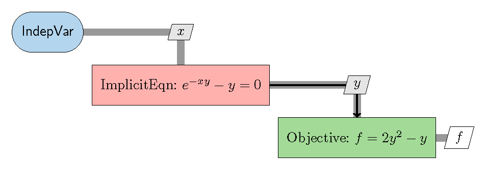
Fig. 1. Example eXtended Design Structure Matrix (XDSM).

Below are the pieces of the runScript.py, a Python script to solve the above optimization problem. To run this case, simply call python runScript.py from your terminal.

class ImplicitEqn(om.ImplicitComponent):
    def setup(self):
        # define input
        self.add_input("x", val=1.0)
        # define output
        self.add_output("y", val=1.0)

    def setup_partials(self):
        # Finite difference all partials.
        self.declare_partials("*", "*", method="fd")

    def apply_nonlinear(self, inputs, outputs, residuals):
        # get the input and output and compute the residual
        # R = e^(-x * y) - y
        # NOTE: we use [0] here because OpenMDAO assumes all inputs
        # and outputs are arrays. If the input is a scalar, OpenMDAO
        # will create an array that has size 1, so to get its value
        # we have to use [0]
        x = inputs["x"][0]
        y = outputs["y"][0]
        residuals["y"] = np.exp(-x * y) - y

This snippet above defines an implicit component (om.ImplicitComponent). In this case, first design the setup function. This function is where you can add inputs and outputs. This is where you also can define your partials, if necessary. Below that is where you define the setup_partials function. In this case, the line self.declare_partials("*", "*", method="fd") declares the partials of every input w.r.t. every output using the "*" and the partial is calculated using "fd" (finite difference). Other methods are "cs" (complex step) or, by not calling a method, OpenMDAO assumes it will be calculated analytically (in this case, users need to provide functions to compute analytical partials). For an implicit component, we create the apply_nonlinear function to define and calculate the residuals. See Implicit Component Documentation for more information.

class Objective(om.ExplicitComponent):
    def setup(self):

        # define input
        self.add_input("y", val=1.0)

        # define output
        self.add_output("f", val=1.0)

    def setup_partials(self):
        # Finite difference all partials.
        self.declare_partials("*", "*", method="fd")

    def compute(self, inputs, outputs):
        # compute the output based on the input
        y = inputs["y"][0]

        outputs["f"] = 2 * y * y - y + 1

The snippet above defines an explicit component (om.ExplicitComponent). Similar to the implicit component, the first steps are defining the setup and setup_partials functions. Now, we define the compute function, where we calculate the outputs. The syntax, as shown in the snippet, must be followed in order for OpenMDAO to recognize the inputs and outputs. If you were to calculate partial derivatives analytically, you will also define a compute_partials function and then run the calculations. See Explicit Component Documentation for more information.

# create an OpenMDAO problem object
prob = om.Problem()
# Add independent variable component
prob.model.add_subsystem("dvs", om.IndepVarComp("x", 1.0), promotes=["*"])
# now add the implicit component defined above to prob
prob.model.add_subsystem("ImplicitEqn", ImplicitEqn(), promotes=["*"])
# add the objective explicit component defined above to prob
prob.model.add_subsystem("Objective", Objective(), promotes=["*"])
# set the linear/nonlinear equation solution for the implicit component
prob.model.nonlinear_solver = om.NewtonSolver(solve_subsystems=False)
prob.model.linear_solver = om.ScipyKrylov()
# set the design variable and objective function
prob.model.add_design_var("x", lower=-10, upper=10)
prob.model.add_objective("f", scaler=1)
# setup the optimizer
prob.driver = om.ScipyOptimizeDriver()
prob.driver.options["optimizer"] = "SLSQP"
# setup the problem
prob.setup()
# write the n2 diagram
om.n2(prob, show_browser=False, outfile="n2.html")
# run the optimization
prob.run_driver()

The snippet above defines the OpenMDAO problem and sets the necessary parameters to run the problem. First, you simply make an OpenMDAO problem (om.Problem()).

Next, you add all the subsystems (components) you created. In this case, dvs (independent variable component), ImplicitEqn (implicit component) and Objective (explicit component) are the subsystems. In the line prob.model.add_subsystem("dvs", om.IndepVarComp("x", 1.0), promotes=["*"]), we create an independent variable component named “dvs,” and inside it we name “x” as an independent variable manually and prescribe it some value. We then promote this value using promotes=["*"]. If a variable “x” is promoted, we can refer to it as “x” later, otherwise, we have to use component_name.variable_name, i.e., “dvs.x”. In addition, OpenMDAO will automatically connect all the variables that have the same names. In this case, OpenMDAO will automatically connect the output “y” from the ImplicitEqn to the input “y” for the “Objective” component. If we do not promote “y”, OpenMDAO will treat them as separate variables (“Implicit.y” and “Objective.y”) without auto-connection.

In the line prob.model.add_subsystem("ImplicitEqn", ImplicitEqn(), promotes=["*"]) we add the subsystem to the model (prob.model.add_subsystem), name the subsystem ("ImplicitEqn" – many times the name can be the same as the name you used to define it), provide the OpenMDAO class that corresponds to the subsystem (ImplicitEqn()), and then promote the variables you want to include (promotes=["*"]), which means promote all inputs and outputs – separate flags exist for the inputs and outputs: promotes_inputs=... and promotes_outputs=... if you want to call them separately or only promote certain outputs.

Next, we add the nonlinear and linear solvers (see Solvers for a list of OpenMDAO solvers).

After that, we set the design variable(s) and objective function. Under add_design_var, first name the variable, then, as in this case, you can add an upper and lower bound for the design variable.

Under add_objective, first name the objective function, then, as in this case, you can add a scaler flag to multiply the model value to get a scaled value. Under each of these, a units=... flag can also be added if they need to be specified.

Next, we set the driver to actually run the optimization. Under the options (prob.driver.option["optimizer"]), set the optimizer you choose to use (as a string). Refer to Drivers for a list of drivers and optimizers that OpenMDAO supports.

Finally, we can setup the problem (prob.setup()). As an option, you can generate the n2 diagram. Lastly, to run the problem, we add the final line prob.run_driver() which will run the entire optimization.

Below is an N2, or N-squared, diagram that OpenMDAO outputs when you run a problem. The N2 diagram will output as .html, which can be opened within a web browser. This is an interactive diagram can help you visualize your connections within your optimization framework.

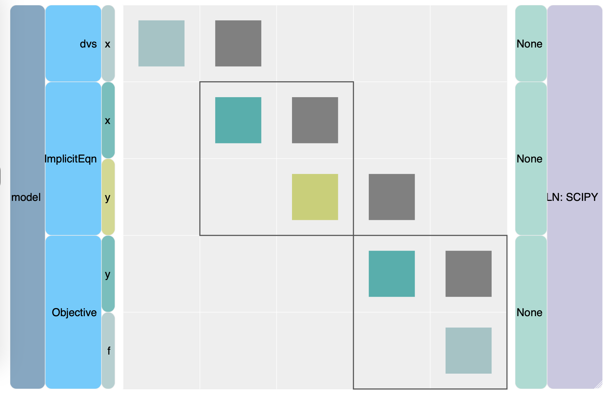
Fig. 2. The N2 diagram for the two-component optimization.

Questions

A factory is designing a cooling system. The system has a controllable design parameter $x$ (for example, the level of power supplied to a fan). This parameter first influences an intermediate system property $z$. The intermediate property then determines the equilibrium value of the system’s temperature $y$, which must be solved implicitly from a nonlinear balance equation. Finally, the overall efficiency cost of the system is computed from the equilibrium temperature and the design parameter. The design goal is to choose the input $x$ that minimizes the cost while also meeting a performance relationship and a safety limit.

The system model is as follows:

Explicit Pre-Process Relation:

The intermediate property $z$ is computed from the design variable:

Implicit Equilibrium Condition:

The equilibrium temperature $y$ must satisfy the nonlinear equation

Explicit Objective Function:

The system cost function is

This design must satisfy the following constraints:

An optimization formulation is given below:

a) Generate the XDSM diagram for the problem. Refer to pyXDSM for the installation and documentation pages.

b) Formulate the problem in OpenMDAO. Use Newton’s method as the nonlinear solver and ScipyKrylov as the linear solver for the implicit system. Use the SLSQP optimizer. Provide the runScript.

c) Generate and show the $N^2$ diagram.

d) Run the optimization and report the optimized $x$, $y$, $z$, and $f$. Verify that the constraints were met. You should arrive that: