pvOptAirfoil is the first in a series of graphical user interface (GUI) plugins that we are developing to streamline the DaFoam optimization process. PvOptAirfoil is designed to make airfoil aerodynamic shape optimization setup more visual throughout the entire process. It can be used for mesh generation and transformation via the DaFOAM Docker image, run-script setup for local optimization using Docker or later exporting to HPC, as well as visualizing optimization results. This GUI is currently in the beta version.
Load the case and plugin
To run a GUI-based optimization case, first download the pvOptGUI tutorial and extract it.
Then, open ParaView following the instructions mentioned on this page.
Then open the pvOptAirfoil source by first clicking the sources tab in the toolbar at the top of the screen. Then hover over pvOptGUI and select pvOptAirfoil. Open a paraview.foam dummy file inside the new source’s file select option, an example of this file is found in pvOptGUI_tutorials.
Then click the green apply button on the left, below the ParaView pipeline window. You can also set up the ‘auto-apply’ feature by navigating to edit in the upper toolbar, then selecting settings. Auto-apply is the second setting under the general tab.
A message box should appear indicating whether a working Docker version was successfully found on your system, click OK
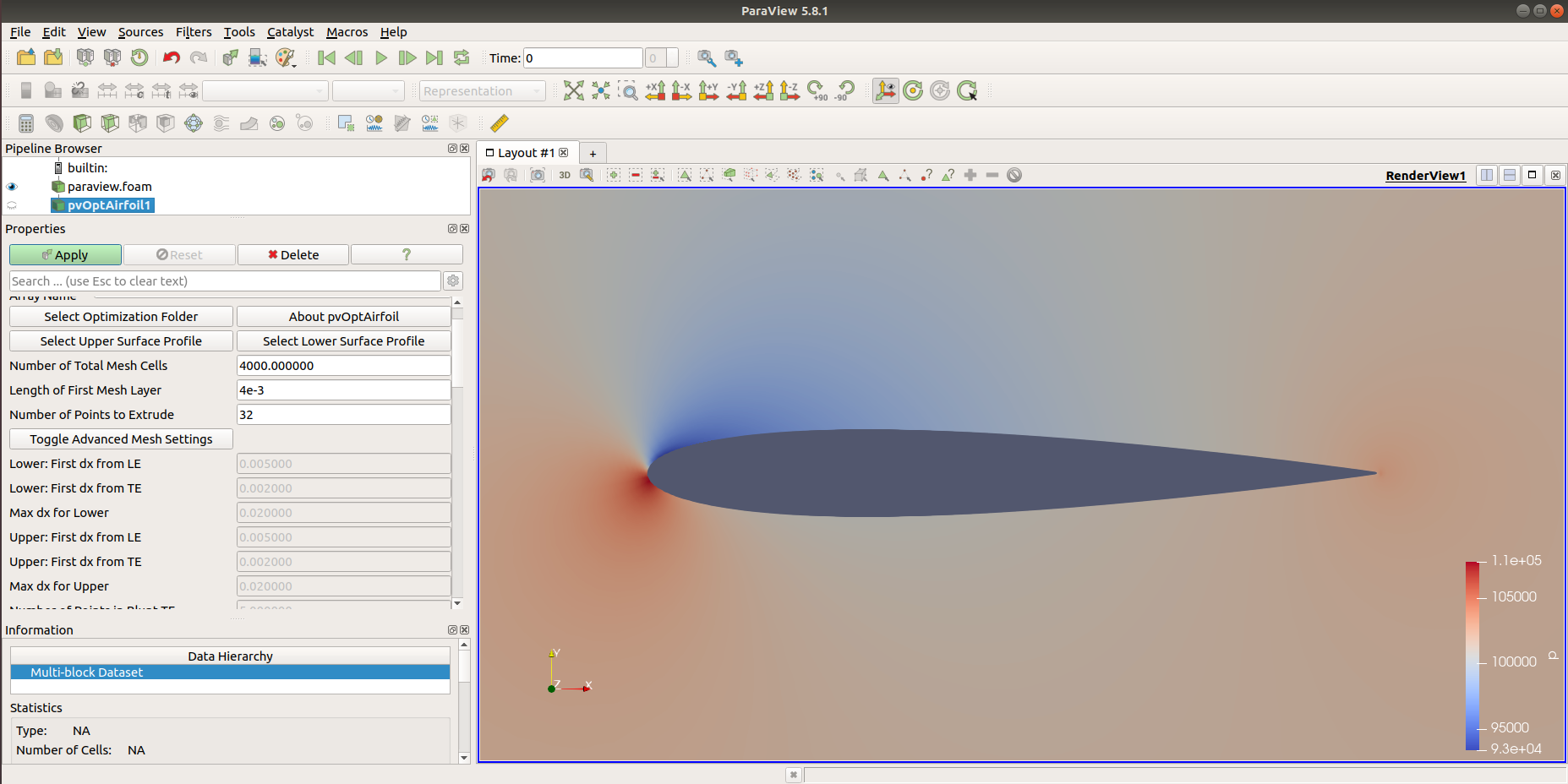
You should now see the pvOptAirfoil interface in the panel on the left, below the pipeline, as shown in the following figure.
Generate the mesh
NOTE: This step requires Docker, if Docker is not found when loading the plugin, the generation files will be created without generating the mesh
First, confirm the optimization folder is selected, then choose the upper and lower profiles for your airfoil by clicking the Select Upper Surface Profile and Select Lower Surface Profile buttons and selecting the files from the dialog. An example of the upper and lower surface profiles can be found pvOptGUI_tutorials/NACA0012/profiles
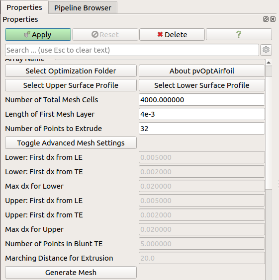
Next you can set the approximate number of mesh cells, the boundary layer thickness and the number of cells between the surface and the far field
Experienced users may choose to select the Toggle Advanced Mesh Settings to refine their mesh further, in which case the total mesh cells is calculated from these inputs
Finally, select the Generate Mesh button to start mesh generation, a few seconds later a message box should appear indicating success or failure and the airfoil’s calculated chord length
NOTE: To load a generated mesh to the viewing area in ParaView, navigate to your paraview.foam file in the pipeline, and click refresh and apply in the menu below (you may need to scroll)
Write the run script
To write the run-script, a number of parameters need to be set
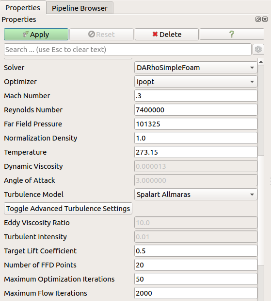
First, select the solver from the dropdown list of supported solvers
- DASimpleFOAM is recommended for mach number below 0.1, incompressible steady-state flow solver for Navier-Stokes equations
- DARhoSimpleFOAM is recommended for mach numbers between 0.1 and 0.6, compressible steady-state flow solver for Navier-Stokes equations (subsonic)
- DARhoSimpleCFOAM is recommended for mach numbers between 0.6 and 1.0, compressible steady-state flow solver for Navier-Stokes equations (transonic)
Select the optimizer from the dropdown list
-
ipopt is the default and is recommended
NOTE: Optimizing with SNOPT requires a license and is not supported for local optimization, more info here
Input the mach number
- You will receive a warning if the input mach number does not match the solver
Input the Reynolds number, a message box will appear asking if you would like to scale the mesh or viscosity, after selection the message box re-appears with the new scaled value
NOTE: Scaling geometry is disabled without Docker and viscosity is scaled automatically
Far Field Pressure
- Not required for DASimpleFOAM solver
Normalization Density
- Not required for DASimpleFOAM solver
Temperature
- Not required for DASimpleFOAM solver
Dynamic Viscosity
- Input disabled, this value is scaled by Reynolds number
Angle of Attack
- Input disabled during optimization setup only, this is an initial condition for the CL Solution, true angle of attack is calculated before optimization by default.
- This option is enabled for flow solution
Select the preferred turbulence model from the dropdown list
- Spalart Allmaras
- K-Omega SST
- K-Epsilon
Experienced users may want to change the turbulence variables. To edit, select the Toggle Advanced Turbulence Settings button
- Eddy Viscosity Ratio
- Turbulent Intensity
NOTE: Some of these variables are not required and are disabled for certain turbulence models
Set target lift coefficient
- This value is used to solve for the angle of attack during the first segment of the optimization
Set number of free form deformation (FFD) points
- These points are distributed outside the airfoil surface and deformed for shape optimization
Set maximum optimization (adjoint) iterations
- The optimization will end if converged before maximum iterations reached
Set maximum (minor) flow iterations
- This limits the number of iterations within each major flow iteration, the individual major iteration will also end if flow converges before maximum iterations reached
Experienced users may wish to change a number of advanced settings in the run-script, to edit the following select the Toggle Advanced Runscript Settings button
- Flow convergence tolerance
- Adjoint convergence tolerance
- Feasibility tolerance
- Optimality tolerance
- Minimum relative thickness
- Maximum relative thickness
- Minimum relative volume
- Maximum relative volume
- The user can also input custom DaOptions, refer to this page for a full list of custom options
NOTE: Preset values in this section are typically sufficient for airfoil optimizations
Finally, you can now click the Generate Runscript button to create the rest of the files required for optimization including the DaFOAM runscript.py, these are created in the optimization folder
NOTE: If values are changed after generating the run-script, simply click the button again to regenerate the files
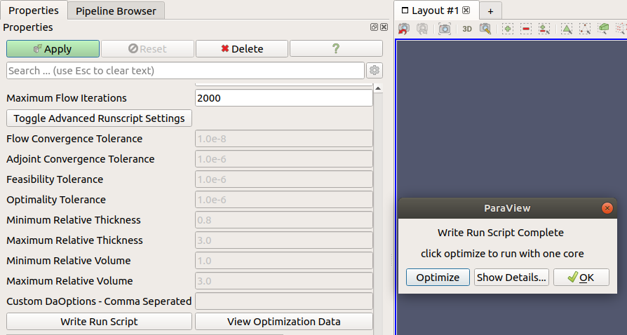
A message box should appear where one can see the full runscript in a small editing window by clicking the Show Details button, accept by clicking OK or run the optimization locally with one core (this requires Docker)
Optimize
After clicking the Write Runscript button at the bottom of the GUI, one should see a message box as described previously. Clicking optimize will run the optimization locally with one core
- If you wish to abort the optimization open the terminal that is currently running paraview (and the optimization) and enter
ctrl+\
Optimization results are output to the file logOpt.txt in your earlier selected optimization folder
A few seconds after starting the optimization, a python GUI will appear showing the optimization results in real time, we recommend making this window full screen
Python GUI for post-processing
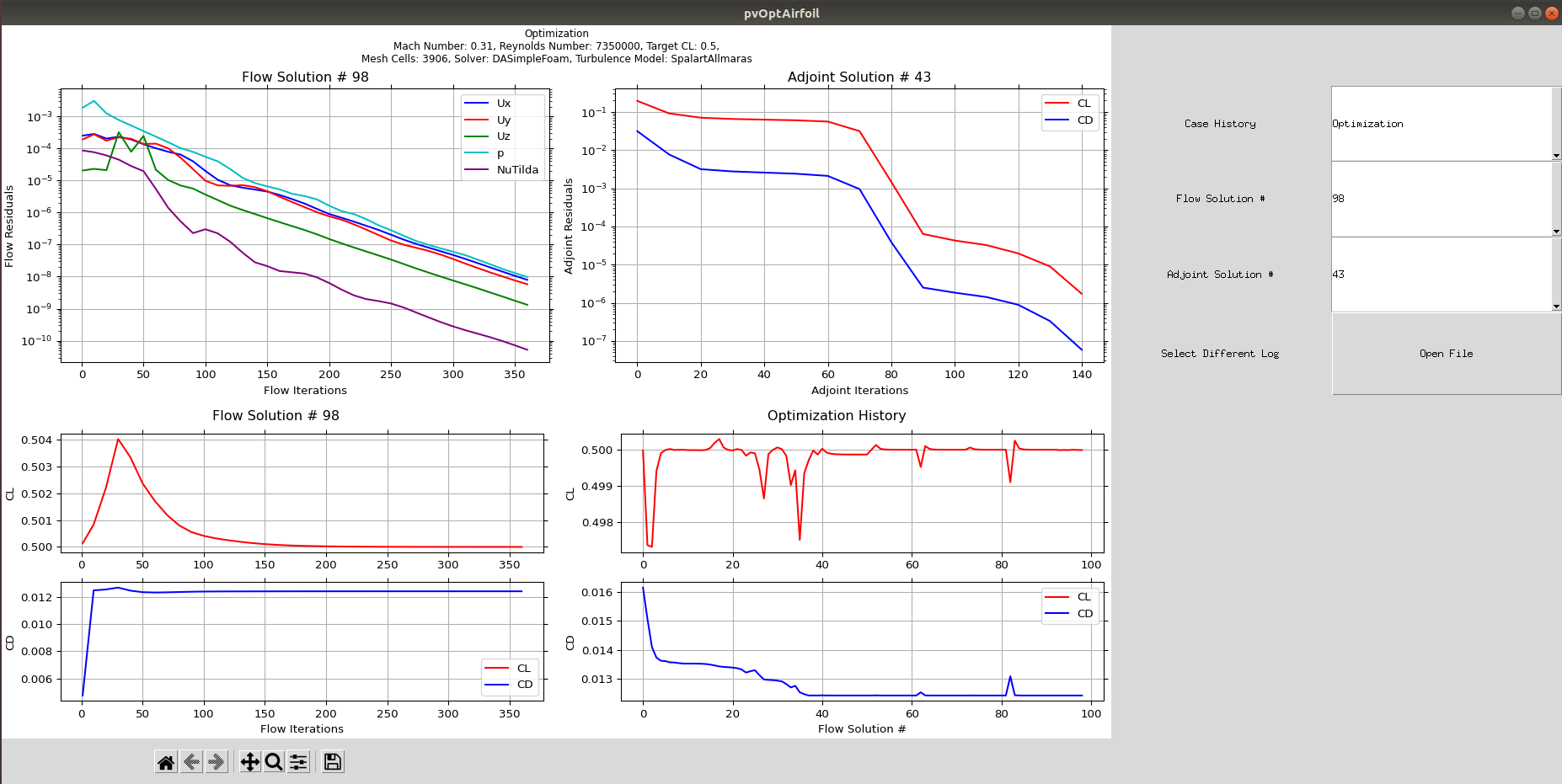
The python script for the post-processing GUI is written to the optimization folder as soon as the folder is selected, this GUI can view optimization results in real time
The python GUI is launched when the optimization starts, but the user can also load the GUI by clicking the View Optimization Data button, located at the bottom of the ParaView interface next to the Write Runscript button. Clicking the View Optimization Data button will automatically load the python GUI with prior data if there is an output logOpt.txt file in the optimization folder. If an optimization is running and the gui has been closed, you can resume viewing optimization results by clicking the View Optimization Data button.
To select a different log file you can click the Open File button on the right hand side of the python GUI
The dropdown box labeled Case History allows one to select the case segment that is being viewed, there are currently two implemented choices that may be contained in your log file
- CL Solution, angle of attack is solved for the target coefficient of lift
- Optimization, selected objective function is optimized
After selecting the portion of the case you wish to view, one can select an adjoint or flow major iteration number
For every adjoint iteration in the optimization there can be several flow iterations
- Loading a flow iteration will load the corresponding adjoint iteration
- Loading an adjoint iteration will load the last corresponding flow iteration
The python GUI also implements the standard Matplotlib toolbar to manipulate plots and export data