This chapter was written by Christian Psenica and reviewed by Ping He.
For more details on the implementation of conjugate heat transfer in DAFoam, please see the following paper:
C. Psenica, L. Fang, S. Zoppelt, M. Leader, P. He. A Modular Conjugate Heat Transfer Optimization Framework for Thermal Management of Electric Aircraft. International Journal of Heat and Mass Transfer, 2026.
Learning Objectives:
This chapter provides the case structure for conjugate heat transfer (CHT) shape optimization in DAFoam. After reading this chapter, you should be able to:
- Describe how to implement two separate domains (fluid and solid) into a DAFoam CHT case
- Describe how the two domains transfer thermal data between eachother
Overview of the U-bend pipe CHT optimization case
This optimization is of a U-bend heat exchanger pipe, shown in Fig. 1. There is a solid domain (the pipe itself) as well as the inner fluid domian (air flowing within the pipe) and external fluid domain (air flowing over the outer surface of the pipe).
Case: U-bend conjugate heat transfer
Geometry: U-bend pipe with circular cross section
Objective function: Pressure loss (minimize) and heat flux (maximize)
Design variables: 36 free-form deformation (FFD) points moving in the x, y, and z directions
Mach number: 0.015 (5 m/s)
Reynolds number: 28,000
Mesh cells: ~788,000
Solver: DASimpleFoam
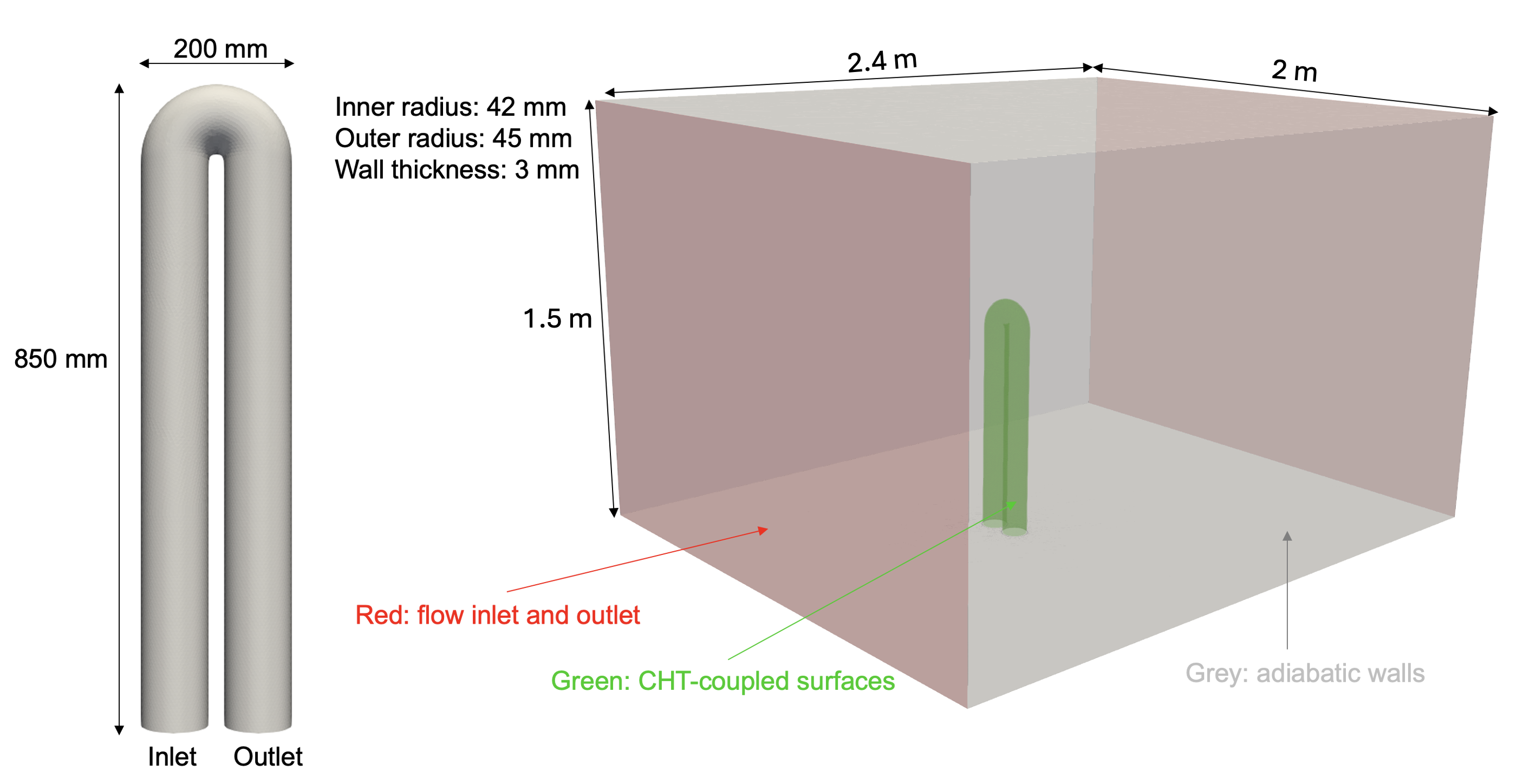
Fig. 1. Schematic of the U-bend heat exchanger configuration
Below is the file and directory structure for the U-bend CHT case in the DAFoam tutorials.
To run the optimization, first run preProcessing.sh to generate the mesh. Then run runScript.py for the optimization. If you wish to re-run the optimizaion, make sure to run Allclean.sh first.
The fluid (aero) domain is very similar to other cases we have shown in previous chapters. In light of this, we will focus on the new parts of this setup, namely, the solid (thermal) domain as well as how to handle multiple domains within runScript.py.
UBend_CHT
|-- aero              # fluid domain configuration files
  |-- 0.orig          # solid domain boundary and initial conditions
  |-- FFD             # free form deformation points
  |-- constant        # flow and turbulence property definition
  |-- system          # flow discretization and setup
  |-- paraview.foam   # dummy file for post processing the fluid domain
|-- thermal           # solid domain configuration files
  |-- 0.orig          # solid domain boundary and initial conditions
  |-- constant        # solid properties (define thermal conductivity)
  |-- system          # thermal discretization and setup
  |-- paraview.foam   # dummy file for post processing the thermal domain
|-- Allclean.sh       # script to clean up the simulation and optimization results
|-- preProcessing.sh  # generate mesh, copy the initial and boundary conditions to 0
|-- runScript.py      # main run script for DAFoam
Solid Domain
0.orig
Similar to previous cases, the 0.orig directory contains the initial and boundary conditions for our field values. It should be noted, however, that the solid domain is a conduction heat transfer problem. Therefore, there is only one field value, the temperature (distribution) of the pipe itself.
The U-bend pipe has four surfaces which need to be specified: the inner surface of the pipe (ubend_inner_solid), the outer surface of the pipe (ubend_outer_solid), and the wall surface of the pipe at the inlet and outlet (inlet_solid and outlet_solid). For this optimization case, we have two sets of CHT interfaces (inner and outer surfaces of the pipe) which take on the mixed (also known as robin type) boundary condition. We use this type of boundary condition as we must balance between temperature and heat flux at the CHT interface. The two wall surfaces at the inlet and outlet are left as zero gradient since this pipe is representative of a system of pipes. This means the pipe is connected to a pump system which pumps fluid through mutliple U-bends, not just one.
dimensions      [0 0 0 1 0 0 0];
internalField   uniform 300;

boundaryField
{
    "(ubend_inner_solid|ubend_outer_solid)"
    {
        type            mixed;
        refValue        uniform 300;
        refGradient     uniform 0;
        valueFraction   uniform 1;
    }

    "(inlet_solid|outlet_solid)"
    {
        type            zeroGradient;
    }
}
constant
As is the case with the system directory, the constant directory only needs to specify information about the pipe material itself. Hence, the only file needed in this directory is solidProperties where we specify the thermal conductivity, $k$, of the material. We simulate an aluminum pipe which has a thermal conductivity of $k=\sim200$ $\frac{W}{m*K}$. Hence in solidProperties we only see:
k 200;
system/controlDict
controlDict for the solid domain is similar to that of the fluid domain but each controlDict is completely stand alone. Below is the controlDict for the solid domain:
startFrom         startTime;
startTime         0;
stopAt            endTime;
endTime           2000;
deltaT            1;
writeControl      timeStep;
writeInterval     2000;
purgeWrite        0;
writeFormat       ascii;
writePrecision    16;
writeCompression  on;
timeFormat        general;
timePrecision     16;
runTimeModifiable true;

DebugSwitches
{
    SolverPerformance 0;
}
For the solid domain we set the endTime to 2000 seconds which is less than the fluid domain. This is typical as the solid domain is easier to converge and therefore requires less iterations to solve. This endTime can be lowered to save computational time.
system/fvSchemes
fvSchemes for the solid domain, shown below for this U-bend case, is a simplified version seen from the fluid domain. This is a steady state analysis so ddtSchemes is set to steadyState.
ddtSchemes
{
    default         steadyState;
}

gradSchemes
{
    default         Gauss linear;
    grad(T)         Gauss linear;
}

divSchemes
{
    default         none;
}

laplacianSchemes
{
    default         none;
    laplacian(k,T)  Gauss linear corrected;
}

interpolationSchemes
{
    default         linear;
}

snGradSchemes
{
    default         corrected;
}
Additionally, since we only have temperature in the solid domain the only gradScheme to set is for temperature where we use Gauss linear. The conduction heat solver does not have any divergence terms and hence the default value is set to none. For laplacianSchemes we only need to specify which scheme to use for laplacian(k,T) which we assign a corrected scheme, Gauss linear corrected. Lastly, for interpolationSchemes we use the standard linear scheme and corrected for snGradSchemes. It should be noted that wallDist is missing. This is used by the turbulence models to compute the distance from the wall. Since there is no turbulence in the solid domain, this option is not needed.
system/fvSolution
fvSolution for the solid domain only needs to contain solver information for temperature. For this, we select the PCG solver with DIC as the preconditioner.
solvers
{
    T
    {
        solver          PCG;
        preconditioner  DIC;
        tolerance       1e-16;
        relTol          1e-4;
        maxIter         3000;
    }
}

SIMPLE
{
    nNonOrthogonalCorrectors 0;
}
The solid domain has a high quality mesh so nNonOrthogonalCorrectors is set to 0.
runScript.py
Most of the changes needed to run a CHT simulation in DAFoam up to this point have the addition of simplified configuration files. Most of the necessary changes to run this case lie within the runScript.py. Here, we must define daOptions for both domains. The first domain we define daOptions for is the fluid domain:
daOptionsAero = {
    #---------- DaOptions Parameters ----------
    "solverName"          : "DASimpleFoam",
    "designSurfaces"      : ["ubend_inner" , "ubend_outer"],
    "useAD"               : {"mode": "reverse"},
    "primalMinResTol"     : 1e-12,
    "primalMinResTolDiff" : 1e11,
    "wallDistanceMethod"  : "daCustom",

    "primalBC" : {
        "U0": {"variable": "U" , "patches": ["inlet"] , "value": [0.0 , U , 0.0]},
        "U1": {"variable": "U" , "patches": ["farfield_inlet"] , "value": [0.0 , 0.0 , -Uf]},
        "p0": {"variable": "p" , "patches": ["outlet"], "value": [p0]},
        "p1": {"variable": "p" , "patches": ["farfield_outlet"], "value": [p0]},
        "nuTilda0": {"variable": "nuTilda", "patches": ["inlet"], "value": [nuTilda0]},
        "nuTilda1": {"variable": "nuTilda", "patches": ["farfield_inlet"], "value": [nuTilda0]},
        "useWallFunction": True,
    },

    #---------- Objective Function ----------
    "function": {

        "TP1": {
            "type"         : "totalPressure",
            "source"       : "patchToFace",
            "patches"      : ["inlet"],
            "scale"        : 1.0,
            "addToAdjoint" : True,
        },

        "TP2": {
            "type"         : "totalPressure",
            "source"       : "patchToFace",
            "patches"      : ["outlet"],
            "scale"        : 1.0,
            "addToAdjoint" : True,
        },

        "Tmean": {
            "type"         : "patchMean",
            "source"       : "patchToFace",
            "patches"      : ["outlet"],
            "varName"      : "T",
            "varType"      : "scalar",
            "component"    : 0,
            "scale"        : 1.0,
            "addToAdjoint" : True,
        },

        "HFX": {
            "type"         : "wallHeatFlux",
            "source"       : "patchToFace",
            "byUnitArea"   : False,
            "patches"      : ["ubend_inner"],
            "scale"        : 1.0,
            "addToAdjoint" : False,
        },

    },

    #---------- Optimization Parameters ----------
    "adjStateOrdering" : "cell",

    "normalizeStates": {"U"       : U ,
                        "p"       : (U * U) / 2. ,
                        "nuTilda" : 1.5e-3 ,
                        "phi"     : 1.0 ,
                        "T"       : 300},

    "adjEqnOption": {"gmresRelTol"         : 1.0e-2,
                     "gmresTolDiff"        : 1.0e2,
                     "pcFillLevel"         : 2,
                     "jacMatReOrdering"    : "natural",
                     "gmresMaxIters"       : 2000,
                     "gmresRestart"        : 2000,
                     "dynAdjustTol"        : True,
                     "useNonZeroInitGuess" : True},

    #---------- Coupling Info ----------
    "inputInfo": {
        "aero_vol_coords" : {"type": "volCoord", "components": ["solver", "function"]},
        "T_convect": {
            "type"        : "thermalCouplingInput",
            "patches"     : ["ubend_inner" , "ubend_outer"],
            "components"  : ["solver" , "function"],
        },
    },

    "outputInfo": {
        "q_convect": {
            "type"       : "thermalCouplingOutput",
            "patches"    : ["ubend_inner" , "ubend_outer"],
            "components" : ["thermalCoupling"],
        },
    },
}
The options here are similar to previous cases in setup. Two noteable subdictionaries, "inputInfo" and "outputInfo", are different. The fluid domain takes in not only the FFD point displacements but also "T_convect" which is temperature for the fluid domain. The fluid domain outputs "q_convect" which is the heat flux at the boundaries in the fluid domain. This is opposite to the solid domain daOptions:
daOptionsThermal = {
    #---------- DaOptions Parameters ----------
    "designSurfaces"      : ["ubend_inner_solid" , "ubend_outer_solid"],
    "solverName"          : "DAHeatTransferFoam",
    "primalMinResTol"     : 1.0e-12,
    "primalMinResTolDiff" : 1.0e11,
    "wallDistanceMethod"  : "daCustom",
    "discipline"          : "thermal",

    #---------- Objective Function ----------
    "function": {

        "HFXsolid": {
            "type"         : "wallHeatFlux",
            "source"       : "patchToFace",
            "byUnitArea"   : False,
            "patches"      : ["ubend_inner_solid"],
            "scale"        : 1.0,
            "addToAdjoint" : False,
        },

    },

    #---------- Optimization Parameters ----------
    "adjStateOrdering" : "cell",

    "adjEqnOption": {"gmresRelTol"         : 1.0e-3,
                     "gmresTolDiff"        : 1e2,
                     "pcFillLevel"         : 1,
                     "jacMatReOrdering"    : "natural",
                     "gmresMaxIters"       : 1000,
                     "gmresRestart"        : 1000,
                     "dynAdjustTol"        : True,
                     "useNonZeroInitGuess" : True},

    "normalizeStates": {"T" : 300},

    #---------- Coupling Info ----------
    "inputInfo": {
        "thermal_vol_coords" : {"type": "volCoord", "components": ["solver", "function"]},
        "q_conduct": {
            "type"           : "thermalCouplingInput",
            "patches"        : ["ubend_inner_solid" , "ubend_outer_solid"],
            "components"     : ["solver"],
        },
    },

    "outputInfo": {
        "T_conduct": {
            "type"       : "thermalCouplingOutput",
            "patches"    : ["ubend_inner_solid" , "ubend_outer_solid"],
            "components" : ["thermalCoupling"],
        },
    },
}
For the solid domain, there is an input of "q_conduct", the heat flux in the solid domain. "T_conduct", the temperature in the solid domain, serves as the output. This is known as the flux forward temperature back scheme (FFTB).
After daOptions we need to setup the builder to initialize the DASolvers. Since we have two domains, we initiatile the DAFoamBuilder twice, once per domain. We also use the MELD thermal scheme to interpolate temperature between the domains and hence initialize the MeldThermalBuilder with both daOptionsAero and daOptionsThermal. Besides intializing the DAFoamBuilder with both domains, we also add the same subsystems for each domain. For example, we have two separate meshes so we add the mesh subsystem for each mesh (domain). Additionally, when we add the scenario, we also specify parameters for the nonlinear block gauss siedel (NLBGS) and linear block gauss siedel (LNBGS) solvers. These are iterative solvers used for converging the two domains to have the same temperature and heat flux solutions. The last important addition is the final line which adds the objective function.
def setup(self):

    #---------- Initialize Builders ----------
    dafoam_builder_aero = DAFoamBuilder(daOptionsAero , meshOptions , scenario = "aerothermal" , run_directory = "aero")
    dafoam_builder_aero.initialize(self.comm)

    dafoam_builder_thermal = DAFoamBuilder(daOptionsThermal , meshOptions , scenario = "aerothermal" , run_directory = "thermal")
    dafoam_builder_thermal.initialize(self.comm)

    thermalxfer_builder = MeldThermalBuilder(dafoam_builder_aero , dafoam_builder_thermal , n = 1 , beta = 0.5)
    thermalxfer_builder.initialize(self.comm)

    #---------- Add Design Variable Component And Promote To Top Level ----------
    self.add_subsystem("dvs" , om.IndepVarComp() , promotes = ["*"])

    #---------- Add Mesh Component ----------
    self.add_subsystem("mesh_aero" , dafoam_builder_aero.get_mesh_coordinate_subsystem())
    self.add_subsystem("mesh_thermal" , dafoam_builder_thermal.get_mesh_coordinate_subsystem())

    #---------- Add Geometry Component ----------
    self.add_subsystem("geometry_aero" , OM_DVGEOCOMP(file = "aero/FFD/UBendFFD.xyz" , type = "ffd"))
    self.add_subsystem("geometry_thermal" , OM_DVGEOCOMP(file = "aero/FFD/UBendFFD.xyz" , type = "ffd"))

    #---------- Add Scenario (Flow Condition) For Optimization ----------
    '''
    For no thermal (solid) use ScenarioAerodynamic, for thermal (solid) use ScenarioAerothermal
    we pass the builder to the scenario to actually run the flow and adjoint
    '''
    self.mphys_add_scenario(
        "scenario" ,
        ScenarioAeroThermal(aero_builder = dafoam_builder_aero , thermal_builder = dafoam_builder_thermal , thermalxfer_builder = thermalxfer_builder),
        om.NonlinearBlockGS(maxiter = 30 , iprint = 2 , use_aitken = True , rtol = 1e-7 , atol = 2e-2),
        om.LinearBlockGS(maxiter = 30 , iprint = 2 , use_aitken = True , rtol = 1e-6 , atol = 1e-2),
    )

    #---------- Manually Connect Aero & Thermal Between The Mesh & Geometry Components ----------
    self.connect("mesh_aero.x_aero0" , "geometry_aero.x_aero_in")
    self.connect("geometry_aero.x_aero0" , "scenario.x_aero")

    self.connect("mesh_thermal.x_thermal0" , "geometry_thermal.x_thermal_in")
    self.connect("geometry_thermal.x_thermal0" , "scenario.x_thermal")

    #---------- Add Objective Function Component ----------
    self.add_subsystem("OBJ" , om.ExecComp("val = scalePL * (TP1 - TP2) + (scaleTM * Tmean)" , scalePL = {'val' : scalePL , 'constant' : True} , scaleTM = {'val' : scaleTM , 'constant' : True}))
The objective function is a weighted sum between pressure loss in the channel and total heat flux:
$f=0.9\frac{T_{M}}{T_{M_\textrm{ref}}} +0.1\frac{C_{PL}}{C_{PL_\textrm{ref}}}$
The pressure loss ($C_{PL}$) is defined as the difference in pressure between the inlet and the outlet and heat flux is handled by minimizing the average outlet temperature ($T_{M}$). Both values are normalized by the baseline values ($C_{PL_\textrm{ref}}$ and $T_{M_\textrm{ref}}$) and scaled by scalePL = 0.1 and scaleTM = 0.9. This weights the objective function for 90% on heat flux performance and 10% on pressure loss. The values for these baseline values and weights are set at the beginning of runScript.py before daOptions:
TMweight = 0.9
TM_baseline = 305.5 ; PL_baseline = 35.07 - 12.76
scaleTM = TMweight / TM_baseline ; scalePL = (1 - TMweight) / PL_baseline
HFX_baseline = -122.85
The last part of runScript.py is the configure(self) function:
def configure(self):

    #---------- Initialize The Optimization ----------
    super().configure()

    #---------- Get Surface Coordinates From Mesh Component ----------
    points_aero = self.mesh_aero.mphys_get_surface_mesh()
    points_thermal = self.mesh_thermal.mphys_get_surface_mesh()

    #---------- Add Pointset To The Geometry Component ----------
    self.geometry_aero.nom_add_discipline_coords("aero" , points_aero)
    self.geometry_thermal.nom_add_discipline_coords("thermal" , points_thermal)

    #---------- Create Design Variables And Assign Them To FFD Points ----------
    # get FFD points
    pts = self.geometry_aero.nom_getDVGeo().getLocalIndex(0)

    # shapex
    indexList = []
    indexList.extend(pts[7:16 , 1 , :].flatten())
    PS = geo_utils.PointSelect("list" , indexList)
    shapexUpper = self.geometry_aero.nom_addLocalDV(dvName = "shapexUpper" , pointSelect = PS , axis = "x")
    shapexUpper = self.geometry_thermal.nom_addLocalDV(dvName = "shapexUpper" , pointSelect = PS , axis = "x")

    # shapey
    indexList = []
    indexList.extend(pts[7:16 , 1 , :].flatten())
    PS = geo_utils.PointSelect("list" , indexList)
    shapeyUpper = self.geometry_aero.nom_addLocalDV(dvName = "shapeyUpper" , pointSelect = PS , axis = "y")
    shapeyUpper = self.geometry_thermal.nom_addLocalDV(dvName = "shapeyUpper" , pointSelect = PS , axis = "y")

    # shapez
    indexList = []
    indexList.extend(pts[7:16 , 1 , :].flatten())
    PS = geo_utils.PointSelect("list", indexList)
    shapezUpper = self.geometry_aero.nom_addLocalDV(dvName = "shapezUpper" , pointSelect = PS , axis = "z")
    shapezUpper = self.geometry_thermal.nom_addLocalDV(dvName = "shapezUpper" , pointSelect = PS , axis = "z")

    # shapex
    indexList = []
    indexList.extend(pts[7:16 , 0 , :].flatten())
    PS = geo_utils.PointSelect("list" , indexList)
    shapexLower = self.geometry_aero.nom_addLocalDV(dvName = "shapexLower" , pointSelect = PS , axis = "x")
    shapexLower = self.geometry_thermal.nom_addLocalDV(dvName = "shapexLower" , pointSelect = PS , axis = "x")

    # shapey
    indexList = []
    indexList.extend(pts[7:16 , 0 , :].flatten())
    PS = geo_utils.PointSelect("list" , indexList)
    shapeyLower = self.geometry_aero.nom_addLocalDV(dvName = "shapeyLower" , pointSelect = PS , axis = "y")
    shapeyLower = self.geometry_thermal.nom_addLocalDV(dvName = "shapeyLower" , pointSelect = PS , axis = "y")

    # shapez
    indexList = []
    indexList.extend(pts[7:16 , 0 , :].flatten())
    PS = geo_utils.PointSelect("list", indexList)
    shapezLower = self.geometry_aero.nom_addLocalDV(dvName = "shapezLower" , pointSelect = PS , axis = "z")
    shapezLower = self.geometry_thermal.nom_addLocalDV(dvName = "shapezLower" , pointSelect = PS , axis = "z")

    #---------- Add Outputs For The DVs ----------
    self.dvs.add_output("shapexUpper" , val = np.array([0]*shapexUpper))
    self.dvs.add_output("shapeyUpper" , val = np.array([0]*shapeyUpper))
    self.dvs.add_output("shapezUpper" , val = np.array([0]*shapezUpper))

    self.dvs.add_output("shapexLower" , val = np.array([0]*shapexLower))
    self.dvs.add_output("shapeyLower" , val = np.array([0]*shapeyLower))
    self.dvs.add_output("shapezLower" , val = np.array([0]*shapezLower))

    #---------- Connect The Design Variables To The Geometry ----------
    self.connect("shapexUpper" , "geometry_aero.shapexUpper")
    self.connect("shapeyUpper" , "geometry_aero.shapeyUpper")
    self.connect("shapezUpper" , "geometry_aero.shapezUpper")
    self.connect("shapexLower" , "geometry_aero.shapexLower")
    self.connect("shapeyLower" , "geometry_aero.shapeyLower")
    self.connect("shapezLower" , "geometry_aero.shapezLower")

    self.connect("shapexUpper" , "geometry_thermal.shapexUpper")
    self.connect("shapeyUpper" , "geometry_thermal.shapeyUpper")
    self.connect("shapezUpper" , "geometry_thermal.shapezUpper")
    self.connect("shapexLower" , "geometry_thermal.shapexLower")
    self.connect("shapeyLower" , "geometry_thermal.shapeyLower")
    self.connect("shapezLower" , "geometry_thermal.shapezLower")

    #---------- Define The Design Variables To The Top Level ----------
    self.add_design_var("shapexUpper" , lower = -0.04 , upper = 0.04 , scaler = 10.0)
    self.add_design_var("shapeyUpper" , lower = -0.04 , upper = 0.04 , scaler = 10.0)
    self.add_design_var("shapezUpper" , lower = -0.04 , upper = 0.04 , scaler = 10.0)
    self.add_design_var("shapexLower" , lower = -0.01 , upper = 0.01 , scaler = 40.0)
    self.add_design_var("shapeyLower" , lower = -0.01 , upper = 0.01 , scaler = 40.0)
    self.add_design_var("shapezLower" , lower = -0.01 , upper = 0.01 , scaler = 40.0)

    #---------- Add Objective And Constraints ----------
    self.connect("scenario.aero_post.TP1"   , "OBJ.TP1")
    self.connect("scenario.aero_post.TP2"   , "OBJ.TP2")
    self.connect("scenario.aero_post.Tmean" , "OBJ.Tmean")
    self.add_objective("OBJ.val" , scaler = 1.0)
We setup the surface coordinates to the geometry component and define the design variables from our FFD points. For this optimization case, we displace 36 FFD points independently in the x, y, and z directions giving 108 total design variables (Fig. 2).
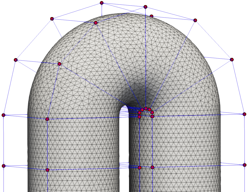
Fig. 2. FFD points used for U-bend CHT optimization
The "upper" design variables are the FFD points along the outer edge of the u-bend while the "lower" design variables are the FFD points along the inner portion of the u-bend. This optimization is unconstrained, so to finalize the configure(self) function we only need to connect the pressure at the inlet and outlet to the corresponding values in the objective function and use add_objective to declare the objective function for optimization.
Questions
TBD