Cylinder - unsteady aerodynamic shape optimization

Edit me

This chapter was written by Zilong Li and reviewed by Ping He.

Learning Objectives:

After reading this chapter, you should be able to:

Setup unsteady aerodynamic shape optimizations

Overview of the Cylinder - unsteady aerodynamic shape optimization

The following is an unsteady aerodynamic shape optimization case for a cylinder

Case: Unsteady flow over a cylinder
Geometry: Cylinder
Objective function: Time-averaged CD
Design variables: 16 FFD points moving in the x direction
Constraints: Cylinder volume does not decrease; FFD symmetry wrt z=0 and y=0
Inlet velocity: 10 m/s
Mesh cells: 2450
Solver: DAPimpleFoam

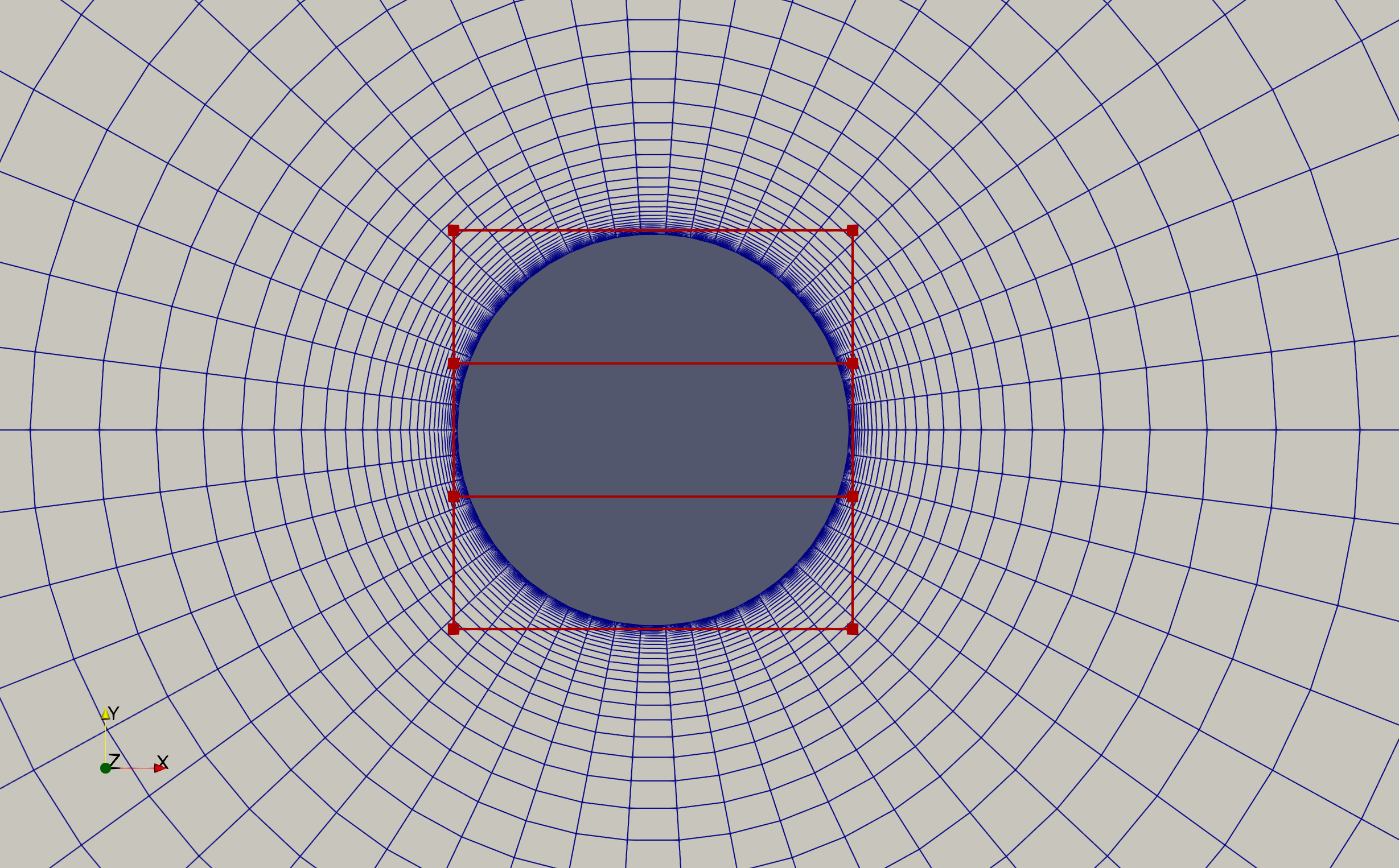
Fig. 1. Mesh and FFD points for the Cylinder case

To run this case, first download tutorials and untar it. Then go to tutorials-main/Cylinder and run the “preProcessing.sh” script to generate the mesh:

./preProcessing.sh

preProcessing.sh

Follow similar steps as in the NACA0012 airfoil case, we use the pyHyp package to generate the mesh. After the mesh generation is done, we are ready to run the simulation. Because in this case we run the unsteady aerodyanmic shape optimization, we need to first run the steady simulation to prepare the initial flow fields for the unsteady optimization. We use the simpleFoam solver to run the steady simulation and reconstruct the flow fields. As a side note, in this case we run the potentialFoam solver to generate the initial flow fields for the simpleFoam.

# run simpleFoam
cp -r system/controlDict_simple system/controlDict
cp -r system/fvSchemes_simple system/fvSchemes
cp -r system/fvSolution_simple system/fvSolution
potentialFoam
mpirun -np 4 python runPrimalSimple.py

# reconstruct the simpleFoam fields
reconstructPar
rm -rf processor*
rm -rf 0
mv 500 0
rm -rf 0/uniform 0/polyMesh

We run simpleFoam for 500 time steps, and after the simpleFoam is done we run the pimpleFoam primal to get equilibrium initial fields. We may need to run pimpleFoam for a long time (10s for this case) to get a stable equilibrium fields, so we copy the content of controlDict_pimple_long to the controlDict.

# run the pimpleFoam primal to get equilibrium initial fields
cp -r system/controlDict_pimple_long system/controlDict
cp -r system/fvSchemes_pimple system/fvSchemes
cp -r system/fvSolution_pimple system/fvSolution
mpirun -np 4 python runScript.py -task=run_model
reconstructPar -latestTime
rm -rf processor*
rm -rf 0
mv 10 0
rm -rf 0/uniform 0/polyMesh
cp -r system/controlDict_pimple system/controlDict

runScript.py

Now let’s elaborate on the runScript.py script, just like the NACA0012 airfoil case, we need to import the necessary modules for DAFoam. Because we run an unsteady optimization here, so we import the DAFoamBuilderUnsteady from dafoam.mphys.mphys_dafoam.

# =============================================================================
# Imports
# =============================================================================
import argparse
import os
import numpy as np
from mpi4py import MPI
import openmdao.api as om
from mphys.multipoint import Multipoint
from dafoam.mphys.mphys_dafoam import DAFoamBuilderUnsteady
from pygeo.mphys import OM_DVGEOCOMP

In the Input Parameters section, the “-optimizer” argument defines the optimizer to use, so we just choose the default “IPOPT” optimizer. The “-task” argument defines the task to run, we run an optimization here, so we set it as “run_driver”. Then we define some global parameters such as “U0”: the far field velocity, “p0”: the far field pressure, “nuTilda0”: the far field turbulence variables, and “A0”: the reference area.

# =============================================================================
# Input Parameters
# =============================================================================
parser = argparse.ArgumentParser()
# which optimizer to use. Options are: IPOPT (default), SLSQP, and SNOPT
parser.add_argument("-optimizer", help="optimizer to use", type=str, default="IPOPT")
# which task to run. Options are: run_driver (default), run_model, compute_totals, check_totals
parser.add_argument("-task", help="type of run to do", type=str, default="run_driver")
args = parser.parse_args()

# Define the global parameters here
U0 = 10.0
p0 = 0.0
nuTilda0 = 4.5e-5
A0 = 0.1

# Set the parameters for optimization
daOptions = {
    "designSurfaces": ["cylinder"],
    "solverName": "DAPimpleFoam",
    "primalBC": {
        "U0": {"variable": "U", "patches": ["inout"], "value": [U0, 0.0, 0.0]},
        "useWallFunction": True,
    },
    "unsteadyAdjoint": {
        "mode": "timeAccurate",
        "PCMatPrecomputeInterval": 100,
        "PCMatUpdateInterval": 1,
        "reduceIO": True,
        "zeroInitFields": False,
    },
    "printIntervalUnsteady": 1,
    "function": {
        "CD": {
            "type": "force",
            "source": "patchToFace",
            "patches": ["cylinder"],
            "directionMode": "fixedDirection",
            "direction": [1.0, 0.0, 0.0],
            "scale": 1.0 / (0.5 * U0 * U0 * A0),
            "timeOp": "average",
        },
        "CL": {
            "type": "force",
            "source": "patchToFace",
            "patches": ["cylinder"],
            "directionMode": "fixedDirection",
            "direction": [0.0, 1.0, 0.0],
            "scale": 1.0 / (0.5 * U0 * U0 * A0),
            "timeOp": "average",
        },
    },
    "adjStateOrdering": "cell",
    "adjEqnOption": {
        "gmresRelTol": 1.0e-100,
        "gmresAbsTol": 1.0e-6,
        "gmresMaxIters": 100,
        "pcFillLevel": 1,
        "jacMatReOrdering": "natural",
        "useNonZeroInitGuess": False,
        "useMGSO": True,
    },
    "normalizeStates": {
        "U": U0,
        "p": U0 * U0 / 2.0,
        "nuTilda": nuTilda0 * 10.0,
        "phi": 1.0,
    },
    "inputInfo": {
        "aero_vol_coords": {"type": "volCoord", "components": ["solver", "function"]},
    },
    "checkMeshThreshold": {"maxAspectRatio": 5000.0},
    "unsteadyCompOutput": {
        "obj": ["CD"],
    },
}

We recommend running this case with 4 CPU cores:

mpirun -np 4 python runScript.py 2>&1 | tee logOpt.txt

We ran this case using the SNOPT optimizer. The case ran for 14 major iterations and took about 10 hours. According to “opt_snopt_summary.txt”, the initial CD is 6.5587285E-01 and the optimized CD is 5.3605074E-01 with a percentage decrease of 18%. Comparison of the unsteady velocity animation and CD time series between the baseline and optimized designs are shown as follows.

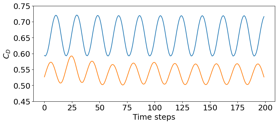
Fig. 2. Time-series of CD for the baseline and optimized design

Fig. 3. Animation of velocity contours for the baseline (left) and optimized (right) designs.