This chapter was written by Ping He.
Learning Objectives:
After reading this chapter, you should be able to:
-
Describe the complete CFD solution workflow for a simple 2D lid-driven cavity problem, including geometry setup, mesh generation, discretization, and solution algorithms.
-
Differentiate between a simple CFD solver and OpenFOAM’s object-oriented implementation.
-
Describe the detailed procedure of the discrete adjoint method using a 1D heat transfer problem, including residual formulation, linearization, and adjoint equation solution.
-
Distinguish between a simple adjoint solver and DAFoam’s Jacobian-free adjoint framework.
Computational Fluid Dynamics (General Introduction)
Computational Fluid Dynamics (CFD) is the numerical solution of the Navier–Stokes (NS) equations that describe fluid motion. The Navier–Stokes equations have no analytical solutions, so we need to solve them on a discretized domain (a mesh). The solution process typically starts with converting the continuous NS equations into the discretized form, reformulate the discretized NS equations into algebraic equations (i.e., matrix-vector product format; Ax=b), and then repeatedly solving large sparse algebraic systems to drive the discretized residuals (R=Ax-b) to zero.
This section shows a simple CFD example by using the finite-volume method to solve steady-state, incompressible, laminar flow in a lid-driven cavity.
1) Governing equations: incompressible, laminar Navier–Stokes (2D)
For this 2D lid-driven cavity example, we solve the incompressible Navier–Stokes equations for a Newtonian fluid with constant density $\rho$ and viscosity $\mu$ in steady state:
Continuity (mass conservation) - 2D \(\frac{\partial u}{\partial x} + \frac{\partial v}{\partial y} = 0\)
Momentum equations (steady) - 2D
$x$-momentum: \(u \frac{\partial u}{\partial x} + v \frac{\partial u}{\partial y} = -\frac{\partial p}{\partial x} + \mu \left( \frac{\partial^2 u}{\partial x^2} + \frac{\partial^2 u}{\partial y^2} \right)\)
$y$-momentum: \(u \frac{\partial v}{\partial x} + v \frac{\partial v}{\partial y} = -\frac{\partial p}{\partial y} + \mu \left( \frac{\partial^2 v}{\partial x^2} + \frac{\partial^2 v}{\partial y^2} \right)\)
where:
- $u(x,y)$ is the horizontal (x-direction) velocity component
- $v(x,y)$ is the vertical (y-direction) velocity component
- $p(x,y)$ is pressure
- No body forces (no gravity, no external forces in this example)
Why is this system difficult?
- Nonlinear: The advection terms $u \frac{\partial u}{\partial x}$ and $v \frac{\partial u}{\partial y}$ make the equations nonlinear
- Coupled: The pressure $p$ is unknown and is determined by the constraint $\nabla \cdot \mathbf{u} = 0$ (continuity). There is no pressure equation, so we must enforce continuity indirectly through a coupling algorithm
2) Discretizing the domain: mesh and control volumes (2D)
For our 2D lid-driven cavity, we use a structured quadrilateral (quad) mesh to discretize the square domain $[0,1] \times [0,1]$.
Mesh concepts for 2D
A mesh partitions the continuous 2D domain into small cells (control volumes). Each cell is a small rectangle where we will store and compute the unknowns ($u, v, p$).
Key mesh terminology in 2D:
-
Mesh cell (control volume): A small rectangular element in the 2D domain. For a uniform quad mesh, all cells are identical. Example: if we have $4 \times 4$ cells, each cell has width and height of $0.25 \times 0.25$ (since domain is $[0,1] \times [0,1]$).
- Mesh face: The boundary edge of a 2D cell. A rectangular cell has exactly 4 faces:
- West face: the left edge (at constant $x$)
- East face: the right edge (at constant $x$)
- South face: the bottom edge (at constant $y$)
- North face: the top edge (at constant $y$)
Each face has an associated length $L_f$ and an outward unit normal vector $\mathbf{n}_f$ (perpendicular to the face, pointing out of the cell).
-
Mesh center (cell center): The geometric center point of a cell $(x_c, y_c)$, where we store the main unknowns: $u(x_c, y_c)$, $v(x_c, y_c)$, and $p(x_c, y_c)$.
Note on storage arrangements: This description assumes a collocated grid, where all variables (velocities and pressure) are stored at the same location (cell centers). An alternative approach is the staggered grid, where velocities are stored at face centers (naturally aligned with flux calculations) and pressure at cell centers. Staggered grids are common in production CFD codes because they provide better pressure-velocity decoupling and reduce numerical oscillations. The CFD implementation example at the end (Section 6) demonstrates a staggered grid approach for this reason.
-
Cell area $A_P$: In 2D, this is the physical area of the cell. For a uniform quad mesh, all cells have the same area. For our example with $n_x \times n_y$ cells: $A_P = \frac{1}{n_x} \times \frac{1}{n_y}$.
- Face flux $\phi_f$: The flow rate (volume per unit time per unit depth) crossing a face. Computed as: $\phi_f = \mathbf{u}_f \cdot \mathbf{n}_f L_f$, where $\mathbf{u}_f = (u_f, v_f)$ is the velocity at the face.
In the above, $n$ is the outward unit normal, and $L_f$ is the face length. In component form: $\phi_f = u_f n_{f,x} L_f + v_f n_{f,y} L_f$
Mesh visualization:
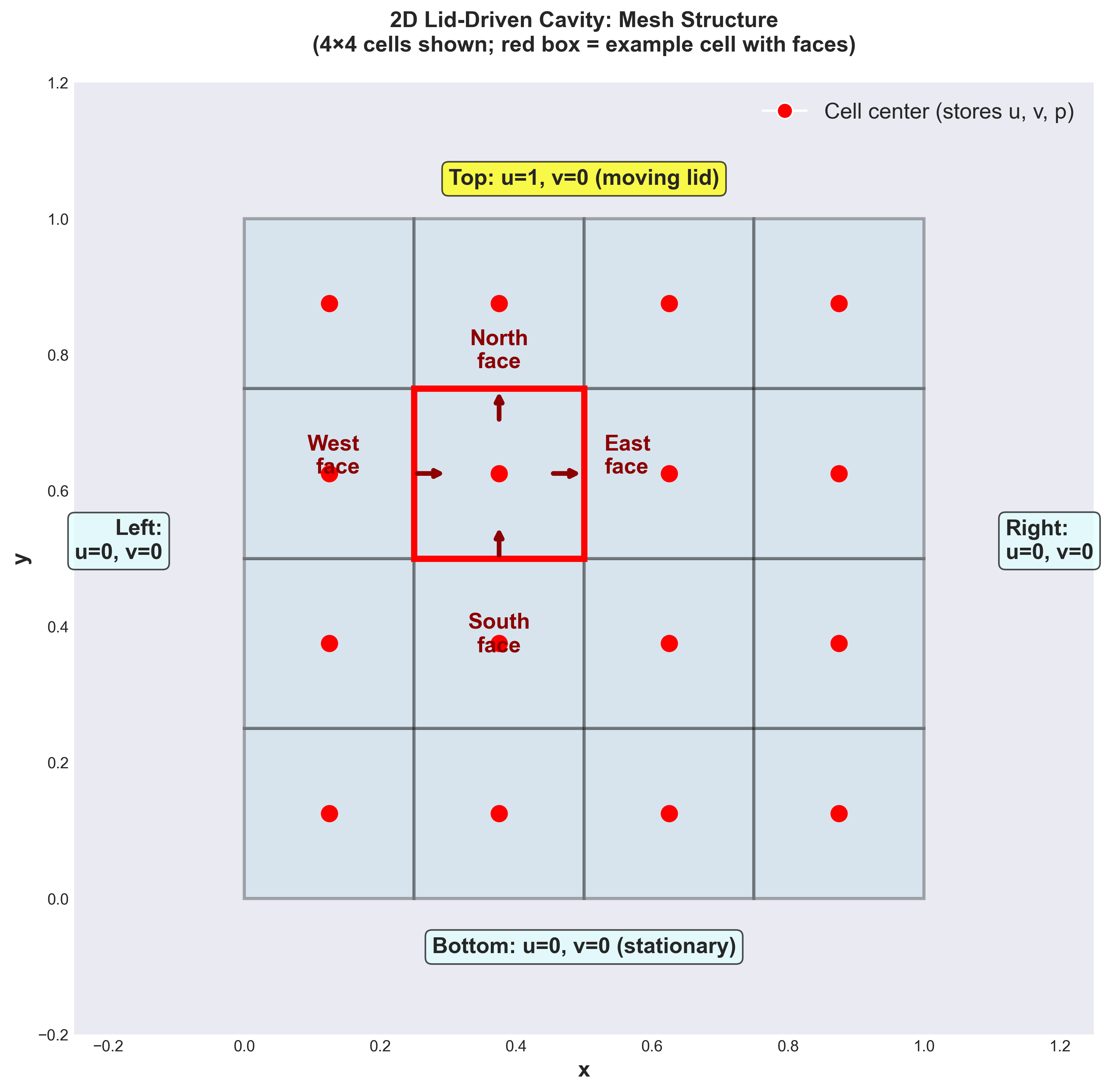
Figure 1: 2D Lid-Driven Cavity Mesh (4×4 cells shown). Red circles (●) mark cell centers where velocity $(u_P, v_P)$ and pressure $p_P$ are stored. The red box highlights one cell and its four faces (east, west, north, south). Boundary conditions are specified on the domain edges: no-slip walls (u=0, v=0) on bottom/left/right, and moving lid (u=1, v=0) on top.
Converting volume to surface integration
Finite-volume CFD stores unknowns as cell-center values (or cell averages) and enforces conservation by balancing fluxes across all faces of each cell. This approach is naturally conservative: what flows out of one cell flows into a neighboring cell.
The divergence theorem (also called Gauss’s theorem or Green’s theorem) converts the volume integral of a divergence into a surface integral: For a scalar $q$ transported by velocity $\mathbf{u}$, integrating over control volume $V_P$: \(\int_{V_P} \nabla\cdot(\mathbf{u}\,q) \, dV = \sum_{f\in \partial V_P} (\mathbf{u}q)_f \cdot \mathbf{n}_f A_f\)
Here $\partial V_P$ denotes the boundary (all faces) of cell $P$.
For a specific cell $P$ in our cavity, the right-hand-side of the above term can be calculated as:
\[\sum_{f\in \partial V_P} (\mathbf{u}q)_f \cdot \mathbf{n}_f A_f = (u_f q_f)_E L_E - (u_f q_f)_W L_W + (v_f q_f)_N L_N - (v_f q_f)_S L_S\]where:
- $(u_f)_E, (u_f)_W, (v_f)_N, (v_f)_S$ are face velocities at the four faces
- $(q_f)_E, (q_f)_W, (q_f)_N, (q_f)_S$ are face scalar variable $q$ at the four faces
- $L_E, L_W, L_N, L_S$ are the face lengths
We can use a similar formulation for other terms in the NS equations. The key insight: the same face flux appears in both adjacent cells with opposite signs. Momentum leaving cell $P$ equals momentum entering its neighbor—automatic conservation.
Flux visualization:
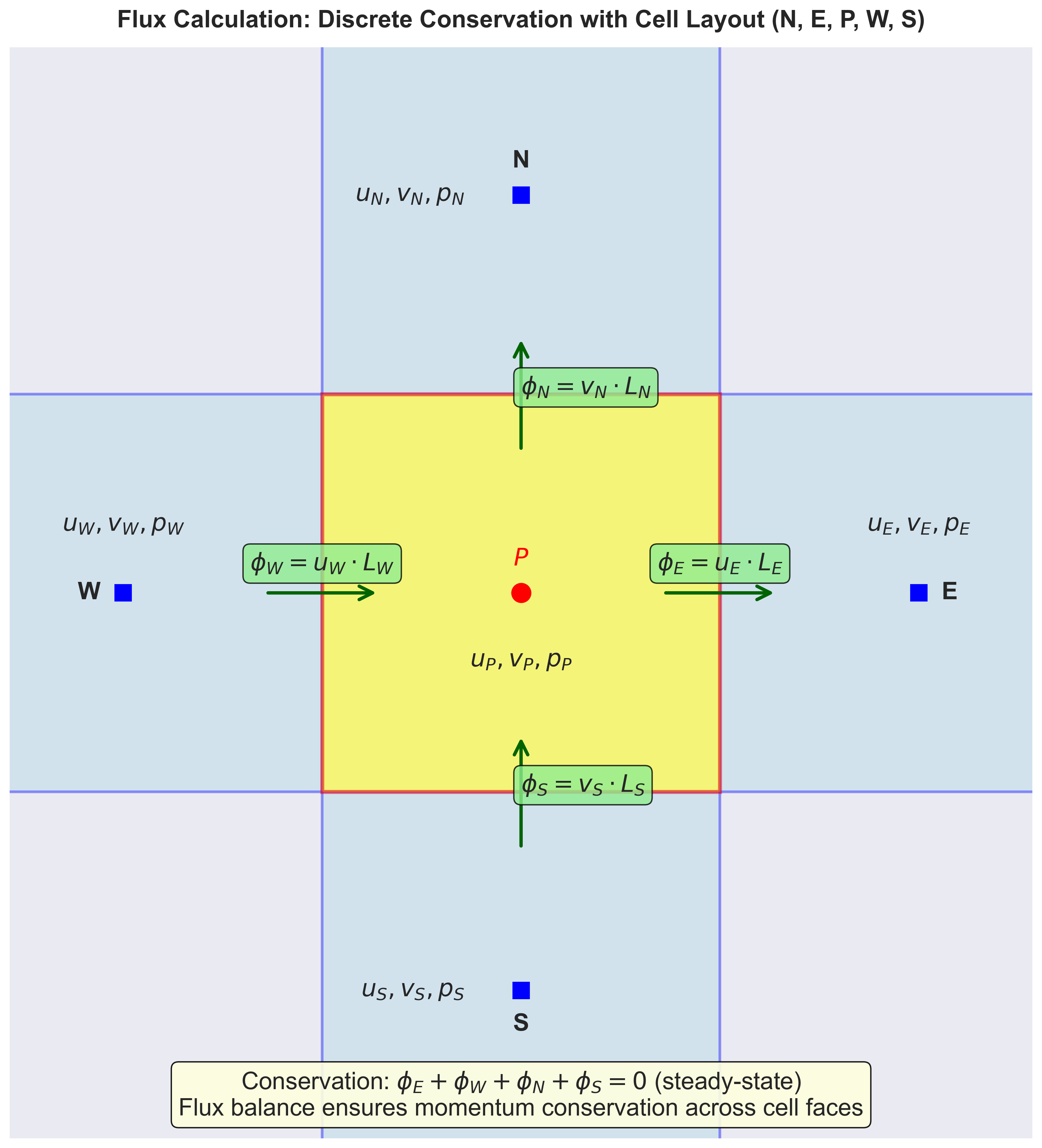
Figure 2: Flux Exchange Between Adjacent Cells. Cell P (yellow, center) exchanges momentum with four neighbors (E, W, N, S) through shared faces. Arrows show the direction of flux at each face. The conservation principle states that the sum of all fluxes must balance: $\phi_E + \phi_W + \phi_N + \phi_S = 0$ in steady state, ensuring what flows out equals what flows in.
3) Turning PDEs into algebra: fluxes, interpolation, and linear systems (2D)
Face values and interpolation (2D example)
Since unknowns are stored only at cell centers, we must interpolate velocity to the cell faces when computing fluxes.
For the 2D lid-driven cavity:
Consider a cell $P$ and its east neighbor $E$. The east face lies halfway between them (at the boundary). To compute the flux through the east face:
- We need $u$ and $v$ at the east face
- These are typically approximated as the average of cell $P$ and cell $E$: \(u_{\text{east face}} = \frac{u_P + u_E}{2}, \quad v_{\text{east face}} = \frac{v_P + v_E}{2}\)
This is a simple linear interpolation (second-order accurate on uniform grids).
For the diffusion terms (viscous terms like $\mu \frac{\partial^2 u}{\partial x^2}$): We compute gradients using central differences between neighboring cell centers. Example:
\[{\frac{\partial u}{\partial x}}\bigg|_{\text{east face}} \approx \frac{u_E - u_P}{\Delta x}\]where $\Delta x$ is the distance between cell centers
Discrete momentum equations in 2D (cell P)
After finite-volume discretization of advection and diffusion, the $x$-momentum equation for cell $P$ becomes a semi-discretized equation (velocity discretization only):
\[a_P u_P^{(n)} = a_E u_E^{(n)} + a_W u_W^{(n)} + a_N u_N^{(n)} + a_S u_S^{(n)} - \frac{\partial p^{(n-1)}}{\partial x}\bigg|_P \cdot A_P\]Similarly for the $y$-momentum equation:
\[a_P v_P^{(n)} = a_E v_E^{(n)} + a_W v_W^{(n)} + a_N v_N^{(n)} + a_S v_S^{(n)} - \frac{\partial p^{(n-1)}}{\partial y}\bigg|_P \cdot A_P\]where: Superscript $(n)$ denotes the current iteration; $(n-1)$ denotes the previous iteration. $a_P, a_E, a_W, a_N, a_S$ are coefficients arising from discretization of advection and diffusion terms. $\frac{\partial p^{(n-1)}}{\partial x}_P$ and $\frac{\partial p^{(n-1)}}{\partial y}_P$ are pressure gradients from the previous iteration (this is the key to the iterative coupling: we use the old pressure to compute the new velocity).
Why is this form useful? It relates the velocity at cell $P$ to its four neighbors (E, W, N, S). This creates a sparse system of linear equations that can be solved iteratively.
The pressure problem: enforcing mass conservation (2D)
In our 2D cavity, there is no explicit equation for pressure. Instead, pressure is determined by requiring that the continuity equation (mass conservation) is satisfied. For steady-state flow, we can derive an equation for pressure as follows:
-
Start with the discretized momentum equations (with coefficients $a_P, a_E, a_W, a_N, a_S$ from advection and diffusion): \(a_P u_P^* = a_E u_E^* + a_W u_W^* + a_N u_N^* + a_S u_S^* + b_P - \frac{\partial p^{(n-1)}}{\partial x}\bigg|_P \cdot A_P\)
-
We can solve the above equation to get the intermediate velocity $\mathbf{u}^* $, which generally does not satisfy continuity: $\nabla \cdot \mathbf{u}^* \neq 0$
-
We enforce the constraint that the corrected velocity must satisfy continuity: \(\nabla \cdot \mathbf{u}^{(n)} = 0 \quad \text{(steady-state incompressible flow)}\)
-
We then make an assumption that the velocity must be corrected by the pressure gradient (momentum equations relate velocity to pressure): \(\mathbf{u}^{(n)} = \mathbf{u}^* - \nabla p^{(n)}\)
-
Substituting into the continuity constraint: \(\nabla \cdot \left( \mathbf{u}^* - \nabla p^{(n)} \right) = 0\)
-
This yields the pressure Poisson equation: \(\nabla^2 p^{(n)} = \nabla \cdot \mathbf{u}^*\)
In discrete form, for each cell $P$: \(\frac{p_E - 2p_P + p_W}{\Delta x^2} + \frac{p_N - 2p_P + p_S}{\Delta y^2} = \frac{u_E^* - u_W^*}{2\Delta x} + \frac{v_N^* - v_S^*}{2\Delta y}\)
This is a sparse symmetric linear system that $p^n$ can be solved using standard solvers (CG, GMRES, multigrid, etc.).
Correcting velocity with the computed pressure:
Once we solve for $p^{(n)}$, we correct the intermediate velocity to enforce continuity:
\[u_P^{(n)} := u_P^* - \frac{p_E^{(n)} - p_W^{(n)}}{2\Delta x}\] \[v_P^{(n)} := v_P^* - \frac{p_N^{(n)} - p_S^{(n)}}{2\Delta y}\]where:
- $u_P^* , v_P^* $ are the intermediate (tentative) velocity components computed from momentum equations with old pressure
- $p^{(n)}$ is the newly computed pressure from the Poisson equation
- $\Delta x, \Delta y$ are grid spacings
This pressure-correction ensures that the new velocity field $\mathbf{u}^{(n)}$ satisfies the continuity constraint to within the tolerance of the Poisson solver. The process repeats (fixed-point iteration) until both momentum and continuity equations are satisfied within specified tolerances.
4) How we solve it: iterative steady-state algorithm (high level)
A typical steady incompressible workflow (SIMPLE-like) looks like:
- Start with initial guesses $\mathbf{u}^{(n-1)}, p^{(n-1)}$
- Solve momentum equations using current pressure to get an intermediate velocity $\mathbf{u}^*$
- Solve a pressure-Poisson equation to get the new pressure $p^n$
- Correct the velocity $u^n$ based on $u^*$ and $p^n$
- Repeat until residuals and mass imbalance are below tolerances
In production codes, each “solve” is a sparse linear solve (e.g., CG, BiCGStab, GMRES with preconditioning), and under-relaxation is often used for stability.
5) Python code to solve the lid-driven cavity flow
Below is a complete Python implementation demonstrating the projection method for steady-state 2D lid-driven cavity flow. This code illustrates the core pressure-velocity coupling algorithm in action:
import numpy as np

def lid_driven_cavity_fv_projection(
    nx=64, ny=64,
    Re=200.0,
    max_iter=5000,
    dt=0.002,
    poisson_iter=80,
    tol_div=1e-6,
    report_every=200
):
    """
    2D incompressible laminar lid-driven cavity (steady solution via pseudo-time stepping).
    Finite-volume projection method on a staggered grid:
      - p at cell centers: (nx, ny)
      - u at vertical faces: (nx+1, ny)  (x-velocity)
      - v at horizontal faces: (nx, ny+1) (y-velocity)

    Domain: [0,1]x[0,1], lid velocity u=1 at top boundary, no-slip elsewhere.
    """

    Lx, Ly = 1.0, 1.0
    dx, dy = Lx/nx, Ly/ny

    rho = 1.0
    nu  = 1.0 / Re  # kinematic viscosity

    # Staggered storage
    p = np.zeros((nx, ny), dtype=float)
    u = np.zeros((nx+1, ny), dtype=float)
    v = np.zeros((nx, ny+1), dtype=float)

    # Helper: enforce velocity boundary conditions (no-slip + moving lid)
    def apply_bc(u, v):
        # u at vertical faces: i=0 and i=nx are left/right walls => u=0
        u[0, :]  = 0.0
        u[-1, :] = 0.0
        # bottom wall (y=0): u=0 at faces adjacent to bottom
        u[:, 0]  = 0.0
        # top lid (y=1): u=1 at faces adjacent to top
        u[:, -1] = 1.0

        # v at horizontal faces: j=0 and j=ny are bottom/top walls => v=0
        v[:, 0]  = 0.0
        v[:, -1] = 0.0
        # left/right walls: v=0 at faces adjacent to left/right
        v[0, :]  = 0.0
        v[-1, :] = 0.0

    apply_bc(u, v)

    # Discrete divergence at cell centers from staggered u,v
    def divergence(u, v):
        # div at p-cells (i=0..nx-1, j=0..ny-1)
        du = (u[1:, :] - u[:-1, :]) / dx
        dv = (v[:, 1:] - v[:, :-1]) / dy
        return du + dv

    # Laplacians for u and v (simple 5-point on their respective grids)
    def lap_u(u):
        Lu = np.zeros_like(u)
        # interior faces for u: i=1..nx-1, j=1..ny-2 (avoid boundaries)
        Lu[1:-1, 1:-1] = (
            (u[2:, 1:-1] - 2*u[1:-1, 1:-1] + u[:-2, 1:-1]) / dx**2 +
            (u[1:-1, 2:]   - 2*u[1:-1, 1:-1] + u[1:-1, :-2]) / dy**2
        )
        return Lu

    def lap_v(v):
        Lv = np.zeros_like(v)
        # interior faces for v: i=1..nx-2, j=1..ny-1
        Lv[1:-1, 1:-1] = (
            (v[2:, 1:-1] - 2*v[1:-1, 1:-1] + v[:-2, 1:-1]) / dx**2 +
            (v[1:-1, 2:] - 2*v[1:-1, 1:-1] + v[1:-1, :-2]) / dy**2
        )
        return Lv

    # Pressure gradients interpolated to u- and v-locations
    def gradp_to_u(p):
        # dp/dx at u-faces (nx+1, ny); interior faces i=1..nx-1
        g = np.zeros((nx+1, ny))
        g[1:-1, :] = (p[1:, :] - p[:-1, :]) / dx
        return g

    def gradp_to_v(p):
        # dp/dy at v-faces (nx, ny+1); interior faces j=1..ny-1
        g = np.zeros((nx, ny+1))
        g[:, 1:-1] = (p[:, 1:] - p[:, :-1]) / dy
        return g

    # Build RHS for pressure Poisson: ∇²p = (rho/dt) * div(u*)
    # Use simple Jacobi iterations for Poisson with Neumann-like behavior at boundaries (dp/dn=0)
    def poisson_pressure(p, rhs):
        pn = p.copy()
        for _ in range(poisson_iter):
            p_old = pn.copy()
            pn[1:-1, 1:-1] = (
                (p_old[2:, 1:-1] + p_old[:-2, 1:-1]) * dy**2 +
                (p_old[1:-1, 2:] + p_old[1:-1, :-2]) * dx**2 -
                rhs[1:-1, 1:-1] * dx**2 * dy**2
            ) / (2*(dx**2 + dy**2))

            # "Neumann" boundaries (zero normal gradient) via copying adjacent interior
            pn[0, :]   = pn[1, :]
            pn[-1, :]  = pn[-2, :]
            pn[:, 0]   = pn[:, 1]
            pn[:, -1]  = pn[:, -2]

            # Fix gauge (pressure defined up to a constant)
            pn[0, 0] = 0.0
        return pn

    for it in range(1, max_iter+1):
        # --- Step 1: tentative velocity u*, v* (explicit convection omitted for simplicity) ---
        # For CFD 101, we keep the core idea: diffusion + pressure projection.
        # Adding convection is straightforward but lengthens the code.
        u_star = u + dt * (nu * lap_u(u) - (1.0/rho) * gradp_to_u(p))
        v_star = v + dt * (nu * lap_v(v) - (1.0/rho) * gradp_to_v(p))

        apply_bc(u_star, v_star)

        # --- Step 2: pressure Poisson from divergence of u* ---
        div_star = divergence(u_star, v_star)
        rhs = (rho/dt) * div_star
        p_new = poisson_pressure(p, rhs)

        # --- Step 3: correct velocities to be divergence-free ---
        u_new = u_star - (dt/rho) * gradp_to_u(p_new)
        v_new = v_star - (dt/rho) * gradp_to_v(p_new)
        apply_bc(u_new, v_new)

        # --- Convergence monitoring: max divergence ---
        div_new = divergence(u_new, v_new)
        max_div = np.max(np.abs(div_new))

        u, v, p = u_new, v_new, p_new

        if (it % report_every) == 0 or it == 1:
            umax = np.max(u); vmax = np.max(v)
            print(f"iter={it:5d}  max|div|={max_div:.3e}  umax={umax:.3f}  vmax={vmax:.3f}")

        if max_div < tol_div:
            print(f"Converged: iter={it}, max|div|={max_div:.3e}")
            break

    # Return fields (staggered) and a cell-centered velocity for convenience
    uc = 0.5 * (u[1:, :] + u[:-1, :])
    vc = 0.5 * (v[:, 1:] + v[:, :-1])
    return uc, vc, p


if __name__ == "__main__":
    uc, vc, p = lid_driven_cavity_fv_projection(nx=64, ny=64, Re=200, max_iter=6000)

    # Optional visualization
    try:
        import matplotlib.pyplot as plt
        nx, ny = p.shape
        x = (np.arange(nx) + 0.5) / nx
        y = (np.arange(ny) + 0.5) / ny
        X, Y = np.meshgrid(x, y, indexing="ij")

        plt.figure()
        plt.contourf(X, Y, p, levels=40)
        plt.colorbar()
        plt.title("Pressure (cell-centered)")

        plt.figure()
        skip = 3
        plt.quiver(X[::skip, ::skip], Y[::skip, ::skip],
                   uc[::skip, ::skip], vc[::skip, ::skip])
        plt.title("Velocity vectors (cell-centered)")
        plt.xlabel("x"); plt.ylabel("y")
        plt.tight_layout()
        plt.show()
    except Exception as e:
        print("Plot skipped:", e)
Key Implementation Concepts:
Note on grid arrangement: This implementation uses a staggered grid arrangement, which differs from the simplified collocated approach described in Section 2 for pedagogical clarity. In the staggered grid:
- Pressure ($p$) is stored at cell centers: shape $(n_x, n_y)$
- Velocity components ($u$, $v$) are stored at face centers:
- $u$ is stored at vertical faces (between cells in x-direction): shape $(n_x+1, n_y)$
- $v$ is stored at horizontal faces (between cells in y-direction): shape $(n_x, n_y+1)$
This arrangement naturally aligns with the face-flux concept (Section 3) and is the standard approach in production CFD codes. It provides better pressure-velocity decoupling and reduces checkerboard oscillations.
Algorithm steps (implementing Section 4):
-
Tentative velocity (Step 1): Compute $\mathbf{u}^*$ using diffusion and current pressure, omitting convection for simplicity.
-
Pressure Poisson (Step 2): Solve $\nabla^2 p^{new} = \frac{\rho}{\Delta t} \nabla \cdot \mathbf{u}^*$ using Jacobi iteration with Neumann-like boundary conditions (zero normal gradient).
-
Velocity correction (Step 3): Update $\mathbf{u}^{new} = \mathbf{u}^* - \frac{\Delta t}{\rho} \nabla p^{new}$ to enforce continuity.
-
Convergence check: Monitor maximum divergence $ \nabla \cdot \mathbf{u} $ at cell centers. When below tolerance ($< 10^{-6}$), the solution has reached steady state. - Pseudo-time stepping: Although the physics is steady (no explicit time dependence), we use small time steps ($\Delta t = 0.002$) to iterate toward steady state, similar to how Section 4 describes a fixed-point iteration for the coupled system.
This minimal code demonstrates the complete pressure-velocity coupling workflow needed to solve incompressible flow, making clear the connection between the general CFD concepts and their implementation.
Computational Fluid Dynamics (OpenFOAM Implementations)
OpenFOAM implements the SIMPLE algorithm (Semi-Implicit Method for Pressure-Linked Equations) using a sophisticated object-oriented framework. While the algorithm remains the same as the 2D cavity example above, OpenFOAM enables seamless handling of complex, industrial-scale problems:
- Unified discretization framework: OpenFOAM uses
fvMatrixto assemble discrete equations systematically; high-level field abstractions (volVectorField,volScalarField) enable intuitive manipulation of finite-volume data across arbitrary 3D meshes - Robust boundary condition handling: Dirichlet, Neumann, and Robin conditions are enforced consistently across all equations through a unified interface
- Modular extensibility: Complex physics (turbulence, heat transfer, multiphase flow) plug into the framework without modifying the core SIMPLE algorithm, enabling rapid development of custom solvers
Initializing runTime and mesh
In OpenFOAM, every application starts by initializing two core objects: runTime and mesh.
runTime object:
- Created by calling
#include "Time.H"in an OpenFOAM solver,runTimeis aTimeobject - Manages time-stepping and I/O control
- Handles time-dependent execution (even for steady-state solvers)
- Controls output directories and time folders
// Access current time value
scalar currentTime = runTime.value();  // Returns current simulation time

// Access time step size
scalar deltaT = runTime.deltaT().value();  // Returns time step Δt

// Access end time (simulation termination criterion)
scalar endTime = runTime.endTime().value();  // Returns target end time

// Increment time and check
runTime++;  // Increments time by deltaT
In CFD context: For steady-state solvers (like lid-driven cavity), runTime essentially manages iteration loops even though there is no physical time. Each “time step” is really an iteration.
mesh object:
- Created by calling
#include "fvMesh.H"in an OpenFOAM solver,meshis afvMeshobject - Represents the computational domain as a structured collection of cells, faces, and vertices
- Stores mesh geometry and connectivity
- Acts as a container for all field data (velocity, pressure, etc.)
Key concept: The mesh object encapsulates the entire finite-volume mesh structure from our general CFD discussion (cells, faces, boundary conditions, etc.). It is the central data structure that OpenFOAM uses to manage all spatial discretization.
// Number of cells and faces
label nCells = mesh.nCells();           // Total number of internal cells
label nFaces = mesh.nInternalFaces();   // Total number of internal faces
label nBoundaryFaces = mesh.nBoundaryFaces();  // Total number of boundary faces

// Cell volumes (corresponds to A_P in CFD)
const Foam::scalarField& V = mesh.V();  // V[cellI] = cell volume (area in 2D)

// Face area vectors (corresponds to L_f · n_f in CFD)
const Foam::surfaceVectorField& Sf = mesh.Sf();  // Sf[faceI] = face area vector

// Cell centers (corresponds to (x_c, y_c) in CFD)
const Foam::vectorField& C = mesh.C();  // C[cellI] = (x_c, y_c, z_c)

// Face centers
const Foam::vectorField& Cf = mesh.Cf();  // Cf[faceI] = (x_f, y_f, z_f)

// Mesh vertices (corner points of cells)
const Foam::pointField& points = mesh.points();  // points[pointI] = (x, y, z) coordinates
label nPoints = mesh.nPoints();                  // Total number of mesh vertices

// Neighbor cell access through face addressing
label cellP = 100;                                   // Center cell
label faceE = mesh.faceOwner().find(cellP);        // Find east face of cell P
label neighborCellE = mesh.faceNeighbour()[faceE]; // Get east neighbor

// Example: Loop over all cells and access their properties
for (label cellI = 0; cellI < mesh.nCells(); ++cellI) {
    scalar cellVolume = mesh.V()[cellI];           // Cell volume
    vector cellCenter = mesh.C()[cellI];           // Cell center position
    // Use these in your discretization...
}
CFD equivalence:
mesh.V()= Cell area $A_P$mesh.Sf()= Face area vector $L_f \cdot \mathbf{n}_f$mesh.C()= Cell center $(x_c, y_c)$
Flow variables: storing data on the mesh
In OpenFOAM, all flow variables (velocity U, pressure p, etc.) are field objects stored directly on the mesh. Each field is tied to the mesh and knows about all cells, internal faces, and boundary faces.
Creating velocity and pressure fields:
- All the field variables are created by calling
#include "createFields.H"in an OpenFOAM solver. Uis avolVectorFieldobject: A field of vectors (3D) defined at cell centers (volume-averaged)pis avolScalarFieldobject: A field of scalars defined at cell centers- Each field has two components: internal field + boundary field
Understanding field components
U.internalField() - Internal cell values
Contains the velocity values at all internal cell centers (cells not on the boundary).
In CFD terms: This is the storage for all $u_P$ values for every cell $P$ in the domain.
- Size: equal to the number of internal cells (
mesh.nCells()) - Ordered sequentially (cell 0, 1, 2, …)
- Each value is a vector $(u, v, w)$ storing the three velocity components at that cell center
- These are the primary unknowns solved in the momentum equations
// Access the internal field (all internal cell values)
// Access velocity at a specific cell (e.g., cellI = 100)
label cellI = 100;
// Get velocity vector (u, v, w) at cell 100. U[cellI] is equivalent to U.internalField()[cellI]
vector velocityAtCell = U[cellI];
scalar Ux = velocityAtCell[0];           // x-component of velocity
scalar Uy = velocityAtCell[1];           // y-component of velocity

// Get the cell center coordinates for this cell
vector cellCenterCoord = mesh.C()[cellI];          // Get (x_c, y_c, z_c) for cell 100
scalar cx = cellCenterCoord[0];               // x-coordinate of cell center
scalar cy = cellCenterCoord[1];               // y-coordinate of cell center

// Get cell volume for this cell
scalar cellVol = mesh.V()[cellI];                  // Get cell area (in 2D) or volume (in 3D)
U.boundaryField() - Boundary condition values
Contains velocity values at all boundary cell centers and stores the boundary condition type (Dirichlet, Neumann, cyclic, etc.).
In CFD terms: These are the Dirichlet boundary conditions (no-slip walls, moving lid) specified on the domain boundaries from our lid-driven cavity example.
Structure:
- Multiple patches (e.g., “bottom”, “left”, “right”, “top”)
- Each patch stores BC type and values at all boundary faces
- Example: moving lid patch has
U = (1, 0, 0)(moving at velocity 1 in x-direction) - Boundary values can be accessed similarly to internal values, indexed by face number on that patch
// Get patch names and loop through all boundary patches
const Foam::polyBoundaryMesh& patches = mesh.boundaryMesh();

// Find and access a specific patch (e.g., "lid" patch for the moving lid)
label patchI = patches.findPatchID("lid");

// if patchI >= 0, the name "lid" is found in constant/polyMesh/boundary,
// otherwise patchI = -1 (there is no "lid" patch)
if (patchI >= 0) {
    // Access the velocity field on this patch
    const Foam::fvPatchVectorField& UPatch = U.boundaryField()[patchI];

    // Get number of boundary faces on this patch
    label nBoundaryFaces = UPatch.size();

    // Access velocity at a specific boundary face (e.g., faceI = 10)
    label faceI = 10;
    vector velocityAtBoundaryFace = UPatch[faceI];  // Get velocity at boundary face
    scalar Ux_bc = velocityAtBoundaryFace[0];       // x-component
    scalar Uy_bc = velocityAtBoundaryFace[1];       // y-component

    // Get face center position on boundary
    vector faceCenterCoord = mesh.Cf().boundaryField()[patchI][faceI];
    scalar xf = faceCenterCoord[0];
    scalar yf = faceCenterCoord[1];

    // Get face area vector on boundary
    vector faceAreaVec = mesh.Sf().boundaryField()[patchI][faceI];
    scalar faceArea = mag(faceAreaVec);
}
Connecting mesh data to finite-volume discretization
How OpenFOAM uses these components:
When computing the discrete momentum equation for a cell, OpenFOAM internally:
- Accesses cell values:
U.internalField()[cellI]→ $u_P$ - Accesses neighbor values: through face addressing, gets
U.internalField()[neighborCellI]→ $u_E, u_W, …$ - Accesses face fluxes: Interpolates to faces using
U.internalField()at both sides - Applies boundary conditions: Uses
U.boundaryField()[patchI]for boundary cells - Integrates over volume: Uses
mesh.V()[cellI]for cell volume weighting - Computes face contributions: Uses
mesh.Sf()[faceI]to get face normal and area
Complete mapping to CFD discretization:
| CFD Concept | OpenFOAM Implementation |
|---|---|
| Cell values $u_P, u_E, u_W, u_N, u_S$ | U.internalField()[cellI] and neighbors |
| Boundary values $u_{\text{boundary}}$ | U.boundaryField()[patchI] |
| Cell volume $A_P$ | mesh.V()[cellI] |
| Face area & normal $L_f \mathbf{n}_f$ | mesh.Sf()[faceI] |
| Cell center position $(x_c, y_c)$ | mesh.C()[cellI] |
| Discrete momentum equation assembly | Handled by fvMatrix (Finite-Volume Matrix) |
Building and solving discretized equations: fvMatrix and solvers
OpenFOAM abstracts the finite-volume discretization process through the fvMatrix class, which represents a discretized linear system in the form Ax = b. Rather than manually assembling the matrix, OpenFOAM provides high-level operators that automatically construct the discrete equations.
// Example: Assemble the momentum equation for steady-state cavity flow
// ddt(rho, U)       → time derivative (zero for steady-state)
// div(phi, U)       → convective (advection) term: ∇·(uU)
// laplacian(mu, U)  → diffusive (viscous) term: ∇²u
// grad(p)           → pressure gradient

volVectorField& U = ...;           // Velocity field
volScalarField& p = ...;           // Pressure field
surfaceScalarField& phi = ...;     // Face flux: phi = U·Sf
scalar rho = 1.0;                  // Density
scalar mu = 1.0;                   // Dynamic viscosity

// Assemble the momentum equation
fvVectorMatrix UEqn
(
    fvm::ddt(rho, U)               // Time derivative: ∂(ρU)/∂t
  + fvm::div(phi, U)               // Convection: ∇·(ρUU)
  - fvm::laplacian(mu, U)          // Diffusion (viscous): μ∇²U
);

// Add pressure gradient source (explicit)
UEqn -= fvc::grad(p);              // fvc::grad() is explicit (not part of matrix)

// Solve the momentum equation: UEqn.A() * U = UEqn.H()
// This is equivalent to: a_P * u_P = sum(a_neighbor * u_neighbor) + source
UEqn.solve();                       // Solves the linear system Ax=b internally
Understanding fvMatrix operators:
fvm::(implicit operators) - Add terms to the left-hand side matrix (A):fvm::ddt(rho, U)- Time derivative, creates diagonal matrix termfvm::div(phi, U)- Convective fluxes, couples with neighborsfvm::laplacian(mu, U)- Diffusive fluxes, couples with neighbors- Result: Contributes to a_P (diagonal) and a_E, a_W, a_N, a_S (off-diagonal)
fvc::(explicit operators) - Compute values at current time step (right-hand side b):fvc::grad(p)- Pressure gradient, treated as known source termfvc::div(flux)- Explicit divergence, no matrix coupling- Result: Contributes to b_P (source vector)
The fvMatrix structure internally represents:
After assembly, fvMatrix stores: - Diagonal coefficient: a_P = diagonal() - Off-diagonal coefficients: [a_E, a_W, a_N, a_S, …] - Right-hand side source: b_P = source() - Boundary field contributions
When you call UEqn.solve(), OpenFOAM: 1. Constructs the sparse matrix A from diagonal and off-diagonal coefficients 2. Constructs the right-hand side vector b from source terms 3. Applies boundary conditions to modify A and b 4. Calls a linear solver (BiCGStab, CG, GMRES, etc. with preconditioner) 5. Returns the solution back to U.internalField()
CFD equivalence - From theory to code:
| CFD Discretization | OpenFOAM Code |
|---|---|
| Discrete equation: $a_P u_P = \sum a_{\text{neighbor}} u_{\text{neighbor}} + b_P$ | fvMatrix UEqn(...) |
| Implicit (matrix) terms: $a_P$, $a_E$, etc. | fvm::div(...), fvm::laplacian(...) |
| Explicit (source) terms: $b_P$ | fvc::grad(p) or other source |
| Linear solve: $Ax = b$ | UEqn.solve() |
| Boundary condition enforcement | UEqn.boundaryManipulate(...) (internal) |
Summary: The data flow in OpenFOAM
runTime → manages time stepping and I/O
    ↓
mesh → stores all geometry (cells, faces, connectivity)
    ├─ mesh.V()        → cell volumes (A_P)
    ├─ mesh.Sf()       → face area vectors (L_f · n_f)
    └─ mesh.C()        → cell centers (x_c, y_c)
    ↓
U, p → flow fields stored on mesh
    ├─ U.internalField()  → cell-center velocities (u_P, u_E, etc.)
    └─ U.boundaryField()  → boundary conditions
    ↓
fvMatrix assembly → builds discrete equations using mesh data
When you write OpenFOAM solvers, you’re working directly with these objects to implement the finite-volume discretization and solvers described in the general CFD section.
Discrete Adjoint Method (1D Example)
The adjoint method is elegant in its mathematical formulation, but the detailed implementation can be non-intuitive. Here we use a 1D diffusion example to showcase exactly how the steady-state adjoint method is implemented step-by-step, from solving the forward problem to computing sensitivities.
Problem description: 1D Diffusion with Nonlinear Source
Consider a one-dimensional diffusion system described by the steady-state PDE:
\[\frac{\partial^2 T}{\partial x^2} - \alpha T^2 = 0\]where:
- $T(x)$ is the temperature field
- $x$ is the spatial coordinate in $[0, 1]$
- $\alpha(x)$ is a spatially varying parameter (design variable)
- All quantities are non-dimensional
Boundary conditions:
- $T(0) = 0$ (left boundary)
- $T(1) = 1$ (right boundary)
This is a nonlinear problem due to the $T^2$ term. We discretize it using finite differences on 11 nodes ($x_0, x_1, \ldots, x_{10}$) with uniform spacing $\Delta x = 0.1$.
Domain discretization:
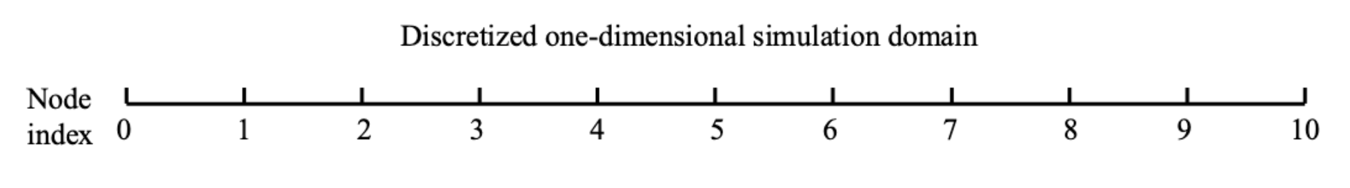
Figure 3: 1D Diffusion Domain Discretization. The domain [0, 1] is discretized into 11 nodes with uniform spacing Δx = 0.1. Boundary conditions are fixed at x₀ = 0 and x₁₀ = 1. Interior nodes (i = 1 to 9) use a 3-point central difference stencil to discretize the PDE. The parameter α is defined at each interior node as a design variable.
Finite-Difference Discretization
We discretize the PDE on all 11 nodes. The discrete residual system $\mathbf{R}(\mathbf{T}, \boldsymbol{\alpha}) = \mathbf{0}$ is a vector of size 11 (one residual per node):
Interior nodes ($i = 1, 2, \ldots, 9$): Use a 3-point central difference stencil:
\[R_i(\mathbf{T}, \boldsymbol{\alpha}) = \frac{T_{i+1} - 2T_i + T_{i-1}}{\Delta x^2} - \alpha_i T_i^2 = 0\]Boundary nodes ($i = 0, 10$): Enforce the Dirichlet boundary conditions directly as constraints:
\(R_0(\mathbf{T}) = T_0 - 0 = 0\) \(R_{10}(\mathbf{T}) = T_{10} - 1 = 0\)
The full discrete system is:
\[\mathbf{R}(\mathbf{T}, \boldsymbol{\alpha}) = \begin{bmatrix} T_0 \\ \frac{T_2 - 2T_1 + T_0}{\Delta x^2} - \alpha_1 T_1^2 \\ \frac{T_3 - 2T_2 + T_1}{\Delta x^2} - \alpha_2 T_2^2 \\ \vdots \\ \frac{T_{10} - 2T_9 + T_8}{\Delta x^2} - \alpha_9 T_9^2 \\ T_{10} - 1 \end{bmatrix} = \mathbf{0}\]This is a system of 11 equations in 11 unknowns ($\mathbf{T}$ of size 11). Given the parameter field $\boldsymbol{\alpha}$, we solve for the temperature field $\mathbf{T}$ (size 11).
Forward Problem: Solving for Temperature
The forward problem solves the nonlinear system iteratively. Given $\alpha(x) = 20$ (constant), the direct method or fixed-point iteration converges to a solution $\mathbf{T}^*$.
Problem Formulation: State, Design, and Objective
Before discussing the adjoint method, we must clearly identify the three key components of this optimization problem:
State Variables (unknowns we solve for):
- $\mathbf{T} = [T_0, T_1, \ldots, T_{10}]^T$ — the temperature at each node
- These satisfy the constraints: $\mathbf{R}(\mathbf{T}, \boldsymbol{\alpha}) = \mathbf{0}$
- Given a choice of $\boldsymbol{\alpha}$, $\mathbf{T}$ is uniquely determined by solving the forward problem
Design Variables (parameters we want to optimize):
- $\boldsymbol{\alpha} = [\alpha_0, \alpha_2, \ldots, \alpha_{10}]^T$ — the nonlinear source coefficient at each node
- These are the free parameters we can adjust
Objective Function (scalar quantity we want to optimize):
- $F(\mathbf{T}) = \sum_{i=0}^{10} T_i$ — the total heat content (sum of all temperatures)
- This depends on the state variables $\mathbf{T}$
- To find how $F$ changes with respect to $\boldsymbol{\alpha}$, we need: $\frac{dF}{d\boldsymbol{\alpha}}$
The Optimization Goal: Compute the sensitivity: How does the objective function $F$ change when we perturb the design variable $\boldsymbol{\alpha}$?
\[\frac{dF}{d\boldsymbol{\alpha}} \quad \text{(gradient of objective w.r.t. design variables)}\]Adjoint Method for Sensitivity Analysis
The adjoint method computes the total derivative $\frac{dF}{d\boldsymbol{\alpha}}$ efficiently in just two steps:
Step 1: Solve the Adjoint Equation
Given the constraint $\mathbf{R}(\mathbf{T}, \boldsymbol{\alpha}) = \mathbf{0}$, solve for the adjoint variables $\boldsymbol{\psi}$ (size 11):
\[\left(\frac{\partial \mathbf{R}}{\partial \mathbf{T}}\right)^T \boldsymbol{\psi} = \left(\frac{\partial F}{\partial \mathbf{T}}\right)^T\]For our problem: $\frac{\partial F}{\partial \mathbf{T}} = [1, 1, \ldots, 1]^T$, so the RHS is a vector of all ones.
Step 2: Compute Total Derivative (Sensitivity)
Once $\boldsymbol{\psi}$ is computed, the total derivative of the objective with respect to design variables is:
\[\frac{dF}{d\boldsymbol{\alpha}} = \frac{\partial F}{\partial \boldsymbol{\alpha}} - \left(\frac{\partial \mathbf{R}}{\partial \boldsymbol{\alpha}}\right)^T \boldsymbol{\psi}\]For our problem: $\frac{\partial F}{\partial \boldsymbol{\alpha}} = \mathbf{0}$ (objective doesn’t depend directly on $\alpha$). This gives us the total derivative (sensitivities) with only two solves: one forward solve (to get $\mathbf{T}$) and one adjoint solve (to get $dF/d\boldsymbol{\alpha}$).
Jacobian Matrices
We need three Jacobians to implement the adjoint method: the state Jacobian (needed for both forward and adjoint solves), the parameter Jacobian (needed for sensitivity computation), and the objective Jacobian (needed for the adjoint RHS).
1. State Jacobian $\frac{\partial \mathbf{R}}{\partial \mathbf{T}}$ (size $11 \times 11$, tridiagonal):
The entry in row $i$, column $j$ is:
\[\frac{\partial R_i}{\partial T_j} = \begin{cases} 1 & \text{if } i = 0 \text{ (boundary node)} \\ 1 & \text{if } i = 10 \text{ (boundary node)} \\ \\ \frac{1}{\Delta x^2} & \text{if } 1 \leq i \leq 9 \text{ and } j = i-1 \\ -\frac{2}{\Delta x^2} - 2\alpha_i T_i & \text{if } 1 \leq i \leq 9 \text{ and } j = i \\ \frac{1}{\Delta x^2} & \text{if } 1 \leq i \leq 9 \text{ and } j = i+1 \\ \\ 0 & \text{otherwise} \end{cases}\]Explicit matrix form:
\[\frac{\partial \mathbf{R}}{\partial \mathbf{T}} = \begin{pmatrix} 1 & 0 & 0 & 0 & \cdots & 0 & 0 \\ \frac{1}{\Delta x^2} & -\frac{2}{\Delta x^2} - 2\alpha_1 T_1 & \frac{1}{\Delta x^2} & 0 & \cdots & 0 & 0 \\ 0 & \frac{1}{\Delta x^2} & -\frac{2}{\Delta x^2} - 2\alpha_2 T_2 & \frac{1}{\Delta x^2} & \cdots & 0 & 0 \\ 0 & 0 & \frac{1}{\Delta x^2} & -\frac{2}{\Delta x^2} - 2\alpha_3 T_3 & \cdots & 0 & 0 \\ \vdots & \vdots & \vdots & \vdots & \ddots & \vdots & \vdots \\ 0 & 0 & 0 & 0 & \cdots & -\frac{2}{\Delta x^2} - 2\alpha_9 T_9 & \frac{1}{\Delta x^2} \\ 0 & 0 & 0 & 0 & \cdots & 0 & 1 \end{pmatrix}\]2. Parameter Jacobian $\frac{\partial \mathbf{R}}{\partial \boldsymbol{\alpha}}$ (size $11 \times 11$, diagonal):
The entry in row $i$, column $j$ is:
\[\frac{\partial R_i}{\partial \alpha_j} = \begin{cases} 0 & \text{if } i = 0 \text{ or } i = 10 \text{ (boundary nodes)} \\ -T_i^2 & \text{if } 1 \leq i \leq 9 \text{ and } i = j \\ 0 & \text{otherwise} \end{cases}\]Explicit matrix form (diagonal with zeros at boundary rows and columns):
\[\frac{\partial \mathbf{R}}{\partial \boldsymbol{\alpha}} = \begin{pmatrix} 0 & 0 & 0 & 0 & \cdots & 0 & 0 \\ 0 & -T_1^2 & 0 & 0 & \cdots & 0 & 0 \\ 0 & 0 & -T_2^2 & 0 & \cdots & 0 & 0 \\ 0 & 0 & 0 & -T_3^2 & \cdots & 0 & 0 \\ \vdots & \vdots & \vdots & \vdots & \ddots & \vdots & \vdots \\ 0 & 0 & 0 & 0 & \cdots & -T_9^2 & 0 \\ 0 & 0 & 0 & 0 & \cdots & 0 & 0 \end{pmatrix}\]3. Objective Function Jacobian $\frac{\partial F}{\partial \mathbf{T}}$ and $\frac{\partial F}{\partial \boldsymbol{\alpha}}$:
Since the objective is $F = \sum_{i=0}^{10} T_i$:
\[\frac{\partial F}{\partial T_i} = 1 \quad \text{for all } i = 0, 1, \ldots, 10\] \[\frac{\partial F}{\partial \alpha_j} = 0 \quad \text{for all } j = 0, 1, \ldots, 10\]The adjoint equation needs $\left(\frac{\partial F}{\partial \mathbf{T}}\right)^T = [1, 1, \ldots, 1]^T$ (a vector of ones, size 11).
Solution Algorithm
Step 1: Solve forward problem
Given: α(x) = 20.0
Solve: R(T, α) = 0 using direct method or fixed-point iteration
Result: T* (converged temperature field)
Step 2: Compute Jacobian dR/dT at the solution
Evaluate ∂R_i/∂T_j at T = T*
Assemble Jacobian matrix [∂R/∂T]
Step 3: Solve adjoint system
Solve: ([∂R/∂T]^T) ψ = (∂F/∂T)^T
Where ∂F/∂T = [1, 1, ..., 1]^T
Result: ψ (adjoint variables)
Step 4: Compute sensitivities
Evaluate ∂R_i/∂α_j at T = T*
For each parameter α_i:
    df/dα_i = ∂F/∂α_i - (∂R/∂α_i)^T · ψ
            = 0 - (-T_i^2) · ψ_i
            = T_i^2 · ψ_i
Result: dF/dα (sensitivities)
Step 5: Verify with finite-difference
For each parameter α_i:
    Perturb: α_new = α + ε·e_i
    Solve forward problem with α_new → T_new
    Compute: f_new = sum(T_new)
    FD derivative: (f_new - f) / ε
Compare with adjoint result
Python code for the adjoint implementation
Below is a complete Python implementation of the adjoint method for the 1D diffusion problem:
import numpy as np

# ============================================================
# Problem Setup
# ============================================================
L = 1.0           # Domain length [0, 1]
dx = 0.1          # Grid spacing
Nx = int(L / dx) + 1  # Number of nodes (Nx = 11)

# ============================================================
# Step 1: Solve Forward Problem - Compute T from R(T, α) = 0
# ============================================================
def run_model(alpha, num_iterations=30):
    """
    Solve the discrete residual system R(T, α) = 0 using fixed-point iteration.

    Args:
        alpha: Design variables (size Nx = 11)
        num_iterations: Number of fixed-point iterations

    Returns:
        T: State variables (temperature field, size Nx = 11)
    """
    T = np.zeros(Nx)  # Initialize temperature
    A = np.zeros([Nx, Nx])  # Discretization matrix A * T = b
    b = np.zeros([Nx, 1])  # RHS vector

    x = np.linspace(0, L, Nx)

    # Set boundary condition values (constant RHS)
    for i in range(Nx):
        if i == 0:
            b[i] = 0.0  # T[0] = 0 (left BC)
        elif i == Nx - 1:
            b[i] = 1.0  # T[Nx-1] = 1 (right BC)
        else:
            b[i] = 0.0  # Interior nodes: homogeneous RHS

    # Fixed-point iteration: assemble and solve A * T = b repeatedly
    for t in range(num_iterations):
        # Assemble the A matrix at current T
        for i in range(Nx):
            if i == 0:
                # Boundary node: R_0 = T_0, so A[0,0] = 1
                A[i, i] = 1.0
            elif i == Nx - 1:
                # Boundary node: R_Nx-1 = T_Nx-1 - 1, so A = 1
                A[i, i] = 1.0
            else:
                # Interior node: R_i = (T_{i+1} - 2T_i + T_{i-1})/dx² - α_i T_i²
                # Diagonal: dR_i/dT_i = -2/dx² - 2α_i T_i
                A[i, i] = -2.0 / (dx * dx) - 2.0 * alpha[i] * T[i]
                # Upper diagonal: dR_i/dT_{i+1} = 1/dx²
                A[i, i + 1] = 1.0 / (dx * dx)
                # Lower diagonal: dR_i/dT_{i-1} = 1/dx²
                A[i, i - 1] = 1.0 / (dx * dx)

        # Solve linear system: T = A^{-1} · b
        T = np.linalg.solve(A, b).flatten()

    return T


# ============================================================
# Objective Function and Its Jacobians
# ============================================================
def calc_F(T):
    """
    Compute objective: F(T) = sum of all temperatures.

    Returns:
        F: Scalar objective value (scalar)
    """
    return sum(T)


def calc_dFdT(T, alpha):
    """
    Compute objective Jacobian: dF/dT_i = 1 for all i.

    Returns:
        dFdT: Gradient vector (size Nx × 1)
    """
    dFdT = np.ones([Nx, 1])
    return dFdT


def calc_dFdAlpha(T, alpha):
    """
    Compute objective Jacobian: dF/dα_i = 0 for all i
    (objective doesn't depend directly on design variables).

    Returns:
        dFdAlpha: Zero vector (size Nx × 1)
    """
    dFdAlpha = np.zeros([Nx, 1])
    return dFdAlpha


# ============================================================
# Jacobian Matrices
# ============================================================
def calc_dRdT(T, alpha):
    """
    Compute state Jacobian: dR/dT (size Nx × Nx, tridiagonal).
    NOTE: if the governing equation was linear dR/dT = A
    However we have a nonlinear term T^2, so dR/dT != A

    The residual is:
    - R_0 = T_0 (boundary)
    - R_i = (T_{i+1} - 2T_i + T_{i-1})/dx² - α_i T_i² (interior)
    - R_Nx-1 = T_Nx-1 - 1 (boundary)

    Returns:
        dRdT: Jacobian matrix (size Nx × Nx)
    """
    dRdT = np.zeros([Nx, Nx])
    for i in range(Nx):
        if i == 0:
            # Boundary: dR_0/dT_0 = 1
            dRdT[i, i] = 1.0
        elif i == Nx - 1:
            # Boundary: dR_Nx-1/dT_Nx-1 = 1
            dRdT[i, i] = 1.0
        else:
            # Interior node (tridiagonal pattern)
            # dR_i/dT_{i-1} = 1/dx²
            dRdT[i, i - 1] = 1.0 / (dx * dx)
            # dR_i/dT_i = -2/dx² - 2α_i T_i
            dRdT[i, i] = -2.0 / (dx * dx) - 2.0 * alpha[i] * T[i]
            # dR_i/dT_{i+1} = 1/dx²
            dRdT[i, i + 1] = 1.0 / (dx * dx)

    return dRdT


def calc_dRdAlpha(T, alpha):
    """
    Compute parameter Jacobian: dR/dα (size Nx × Nx, diagonal).

    The residual w.r.t. α_j is:
    - dR_0/dα_j = 0 (boundary, doesn't depend on α)
    - dR_i/dα_j = -T_i² if i == j, else 0 (interior, only diagonal)
    - dR_Nx-1/dα_j = 0 (boundary, doesn't depend on α)

    Returns:
        dRdAlpha: Jacobian matrix (size Nx × Nx, diagonal with zeros at boundaries)
    """
    dRdAlpha = np.zeros([Nx, Nx])
    for i in range(Nx):
        if i == 0 or i == Nx - 1:
            # Boundary nodes don't depend on design variables
            dRdAlpha[i, i] = 0.0
        else:
            # Interior nodes: dR_i/dα_i = -T_i²
            dRdAlpha[i, i] = -T[i] ** 2

    return dRdAlpha


# ============================================================
# Step 2 & 3: Solve Adjoint System to get ψ
# ============================================================
# Given: State Jacobian dRdT and objective Jacobian dFdT
# Solve: (dR/dT)^T · ψ = (dF/dT)^T

# Set design variables
alpha = np.ones(Nx) * 20.0  # Uniform parameter field

# Step 1: Solve forward problem
T = run_model(alpha)
print(f"Forward solution T: {T}")

# Step 2: Compute Jacobians
dRdT = calc_dRdT(T, alpha)
dFdT = calc_dFdT(T, alpha)
dRdAlpha = calc_dRdAlpha(T, alpha)
dFdAlpha = calc_dFdAlpha(T, alpha)

# Step 3: Solve adjoint system
# (dR/dT)^T · ψ = (dF/dT)^T
dRdT_transpose = np.transpose(dRdT)
psi = np.linalg.solve(dRdT_transpose, dFdT)
print(f"Adjoint variables ψ: {psi.flatten()}")

# ============================================================
# Step 4: Compute Sensitivities using Adjoint Formula
# ============================================================
# dF/dα = dF/dα (direct term) - (dR/dα)^T · ψ
#       = 0 - (dR/dα)^T · ψ  (since dF/dα = 0)

total_adjoint = dFdAlpha - np.dot(np.transpose(dRdAlpha), psi)
print(f"Adjoint sensitivities dF/dα:\n{total_adjoint.flatten()}")

# ============================================================
# Step 5: Verify with Finite-Difference
# ============================================================
# For each parameter α_j, perturb and recompute objective

F_ref = calc_F(T)  # Reference objective
total_FD = np.zeros(Nx)
eps = 1e-1  # Finite-difference step size

for i in range(Nx):
    # Perturb parameter i
    alpha_perturbed = alpha.copy()
    alpha_perturbed[i] = alpha[i] + eps

    # Solve forward problem with perturbed parameter
    T_perturbed = run_model(alpha_perturbed)

    # Compute new objective
    F_perturbed = calc_F(T_perturbed)

    # Finite-difference derivative: (F(α+ε) - F(α)) / ε
    total_FD[i] = (F_perturbed - F_ref) / eps

print(f"Finite-difference sensitivities dF/dα:\n{total_FD}")
print(f"\nComparison (Adjoint vs FD):")
print(f"  Max difference: {np.max(np.abs(total_adjoint.flatten() - total_FD))}")
This code implements the complete adjoint method workflow:
run_model(): Solves the forward problem (R(T, α) = 0) using fixed-point iterationcalc_dRdT(),calc_dRdAlpha(): Compute required Jacobian matrices- Adjoint solve: Solves $(dR/dT)^T \psi = (dF/dT)^T$ to get adjoint variables
- Sensitivity computation: Uses adjoint variables to compute $dF/d\alpha$ in one pass
- Verification: Compares adjoint results with finite-difference approximation
The adjoint method computes sensitivities for all 11 parameters using only 2 solves (one forward, one adjoint), regardless of parameter count.
Discrete Adjoint Method (DAFoam Implementations)
The 1D diffusion example above demonstrates the core adjoint concepts in a highly simplified case. However, applying adjoint methods to large-scale CFD solver like OpenFOAM introduces significant challenges. DAFoam handle these challenging by using a Jacobian-free adjoint approach, elaborated on as follows.
Unified coupled variables and residual formulation
In the 1D example, we had a scalar state variable $T$ and a single residual equation $R(T, \alpha) = 0$. Real CFD systems involve multiple coupled flow variables:
- Velocity components: $\mathbf{u} = (u, v, w)$ (3 equations)
- Pressure: $p$ (1 equation)
- Turbulence variables: $k$, $\epsilon$, etc. (additional equations for RANS)
All residuals are inter-coupled: momentum equations contain pressure gradients, continuity constrains the divergence of velocity, turbulence models depend on velocity gradients. Carefully defining the coupled residual vector $\mathbf{R}(\mathbf{W}, \mathbf{X})$ becomes non-trivial, where $\mathbf{W}$ are all state variables (velocity, pressure, turbulence) and $\mathbf{X}$ are design variables (mesh, material properties, etc.). Additionally, boundary conditions introduce complications: how do inlet/outlet velocities and pressure affect the Jacobian?
DAFoam’s Solution:
DAFoam leverages OpenFOAM’s fvMatrix class to systematically assemble discrete residuals for all equations:
- Each equation (momentum, continuity, turbulence) is formulated as $\mathbf{A} \mathbf{W} = \mathbf{b}$ where $\mathbf{A}$ is a sparse matrix and $\mathbf{b}$ is the RHS, they are both stored in fvMatrix.
- Boundary conditions are incorporated consistently into $\mathbf{A}$ and $\mathbf{b}$
- The residual is: $\mathbf{R} = \mathbf{A} \mathbf{W} - \mathbf{b}$
- All residuals (momentum, continuity, turbulence) are stacked into a single vector: $\mathbf{R}(\mathbf{W}, \mathbf{X})$
This approach ensures:
- Consistent treatment of Dirichlet, Neumann, and Robin boundary conditions across all equations
- Design variable dependence (e.g., mesh movement affecting cell volumes and face areas) is tracked automatically
Jacobian-free adjoint method
In the 1D example, we explicitly formed and stored the state Jacobian $\frac{\partial \mathbf{R}}{\partial \mathbf{W}}$, a tridiagonal $11 \times 11$ matrix. For large-scale CFD problems with millions of unknowns, explicitly forming and storing this Jacobian is prohibitive in terms of memory and computational cost. Additionally, computing the exact Jacobian requires careful differentiation of complex nonlinear terms (convection, turbulence models), which becomes error-prone and difficult to maintain.
Jacobian-free GMRES approach:
Instead of explicitly computing and storing $\frac{\partial \mathbf{R}}{\partial \mathbf{W}}$, DAFoam uses Jacobian-free GMRES to solve the adjoint equation: \(\left(\frac{\partial \mathbf{R}}{\partial \mathbf{W}}\right)^T \boldsymbol{\psi} = \left(\frac{\partial F}{\partial \mathbf{W}}\right)^T\)
The key insight is that GMRES only requires matrix-vector products of the form $\frac{\partial \mathbf{R}}{\partial \mathbf{W}}^T \mathbf{r}$ during iterations, not the full matrix. GMRES constructs the solution as a linear combination of vectors in the Krylov subspace:
\[K_n = \text{span}\{\mathbf{r}_0, \mathbf{A}\mathbf{r}_0, \mathbf{A}^2\mathbf{r}_0, \ldots, \mathbf{A}^{n-1}\mathbf{r}_0\}\]This accumulates information across all iterations, achieving faster convergence than fixed-point methods.
Computing matrix-vector products via reverse-mode automatic differentiation:
We use reverse-mode automatic differentiation to compute matrix-vector products on-the-fly without forming the Jacobian: \(\overline{\mathbf{w}} = \left(\frac{\partial \mathbf{R}}{\partial \mathbf{W}}\right)^T \overline{\mathbf{R}}\)
where $\overline{\mathbf{R}}$ (with overbar) denotes the input vector to be propagated backward through the adjoint computation, and $\overline{\mathbf{w}}$ (with overbar) is the resulting adjoint output representing the sensitivity with respect to state variables $\mathbf{W}$. In the GMRES iterations, we set $\overline{\mathbf{R}} = \mathbf{r}_0$ (the GMRES residual vector), and the output $\overline{\mathbf{w}} = \left[\frac{\partial \mathbf{R}}{\partial \mathbf{W}}\right]^T \mathbf{r}_0$ is the matrix-vector product we need, all computed without explicitly storing the Jacobian.
Note that we $\frac{\partial F}{\partial \mathbf{W}}$ is also computed via reverse-mode AD.
Preconditioning for ill-conditioned systems:
The state Jacobian from 3D viscous turbulent flow is typically ill-conditioned (high ratio of largest to smallest eigenvalues), causing GMRES to converge slowly. We use a preconditioner matrix $\left[\frac{\partial \mathbf{R}}{\partial \mathbf{W}}\right]^T_{PC}$ to transform the system into a better-conditioned form:
\[\left(\left[\frac{\partial \mathbf{R}}{\partial \mathbf{W}}\right]^T_{PC}\right)^{-1}\left(\frac{\partial \mathbf{R}}{\partial \mathbf{W}}\right)^T \boldsymbol{\psi} = \left(\left[\frac{\partial \mathbf{R}}{\partial \mathbf{W}}\right]^T_{PC}\right)^{-1}\left(\frac{\partial F}{\partial \mathbf{W}}\right)^T\]where $\left[\frac{\partial \mathbf{R}}{\partial \mathbf{W}}\right]^T_{PC} \approx \left[\frac{\partial \mathbf{R}}{\partial \mathbf{W}}\right]^T$ but is much easier to invert. An efficient preconditioner clusters the eigenvalues, dramatically improving GMRES convergence.
To explicitly compute $\left[\frac{\partial \mathbf{R}}{\partial \mathbf{W}}\right]^T_{PC}$, DAFoam uses a heuristic graph coloring approach to accelerate the automatic differentiation computation, which groups variables that can be differentiated simultaneously without dependence conflicts.
DAFoam uses the PETSc software library with a nested preconditioning strategy:
- GMRES (top-level solver)
- Additive Schwarz Method (ASM) (global preconditioner—divides system into overlapping blocks solved in parallel)
- Incomplete LU (ILU) factorization (local preconditioner in each block)
- Richardson iterations (inner and outer iterations to reduce memory cost)
Computing sensitivities with respect to design variables:
Once the adjoint variables $\boldsymbol{\psi}$ are obtained, we compute the total derivative of the objective with respect to design variables $\mathbf{X}$:
\[\frac{dF}{d\mathbf{X}} = \frac{\partial F}{\partial \mathbf{X}} - \left(\frac{\partial \mathbf{R}}{\partial \mathbf{X}}\right)^T \boldsymbol{\psi}\]Again, DAFoam does not use analytical approach. Instead, it uses AD:
-
Direct objective partial: $\frac{\partial F}{\partial \mathbf{X}}$ — computed via reverse-mode AD (typically zero or small if the objective depends only on state variables)
-
Design-dependent residual Jacobian: $\left(\frac{\partial \mathbf{R}}{\partial \mathbf{X}}\right)^T \boldsymbol{\psi}$ — computed using a Jacobian-free approach similar to the adjoint solve. Rather than explicitly forming the matrix, we use reverse-mode AD to compute the product directly, where $\boldsymbol{\psi}$ is propagated backward through the residual computation.
Comparison: 1D Example vs. DAFoam Implementation
The following table highlights the key differences between the simple 1D adjoint method example and DAFoam’s large-scale adjoint implementation:
| Aspect | 1D Diffusion Example | DAFoam CFD Adjoint |
|---|---|---|
| State variables | Single scalar $T$ (11 nodes) | Coupled vectors: velocity, pressure, turbulence (millions of nodes) |
| System size | $11 \times 11$ Jacobian | Could be millions × millions |
| State Jacobian storage | Explicitly formed and stored | Never formed—Jacobian-free approach |
| Adjoint solve method | Direct dense linear solver | GMRES with nested preconditioning (PETSc) |
| Matrix-vector products | Explicit matrix multiply | Reverse-mode AD on-the-fly computation |
| Computing $\frac{\partial \mathbf{R}}{\partial \mathbf{X}}^T \boldsymbol{\psi}$ | Analytical formula | Reverse-mode AD matrix-vector product computation |