MACH Tutorial wing - aero-structural optimization

Edit me

This chapter was written by Ping He.

Learning Objectives:

After reading this chapter, you should be able to:

Identify the main difference in runScript.py between an aerodynamic-only and an aero-structural optimization
Setup and run a new aero-structural optimization case

Overview of the MACH tutorial wing

The following is an aerostructural shape optimization case for the MACH tutorial wing in subsonic conditions. The flow is solved using the DARhoSimpleFoam CFD solver and the structure is solved using an open-source FEM solver TACS. The load and displacement transfer is computed using FUNtoFEM. The aerostructural coupling is implemented in the OpenMDAO/Mphys framework. Here we assume you are familiar with aerodynamic-only optimization for wings, and we will focus on the difference between the aero-only and aerostructural optimization.

Case: Wing aerostructural optimization 
Geometry: MACH tutorial wing
Objective function: Drag coefficient (CD)
Lift coefficient (CL): 0.5
Design variables: 96 FFD points moving in the y direction, seven twists, and one angle of attack.
Constraints: volume, thickness, LE/TE, lift, and stress constraints (total number: 118)
Mach number: ~0.3 (100 m/s)
Reynolds number: ~30 million
Mesh cells: ~38,000
Solver: DARhoSimpleFoam

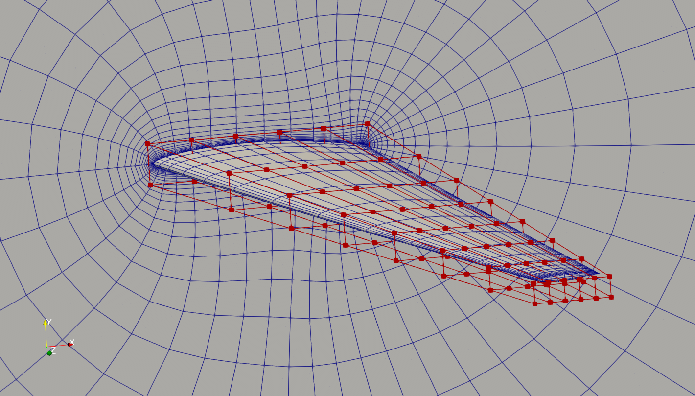
Fig. 1. Mesh and FFD points for the MACH tutorial wing.

Differences in runScript.py

The first main difference is the import of the TACS script

import tacsSetup

Here we import the tacsStep.py file in the working directory for setting up the structural anlysis in TACS.

The first block of the script is to define the material properties, such as density and elastic modules. Here we also define the initial thickness for all the spars and ribs in the wing box, and their corresponding upper and lower bounds (tMin and tMax).

# Material properties
rho = 2780.0  # density, kg/m^3
E = 73.1e9  # elastic modulus, Pa
nu = 0.33  # poisson's ratio
kcorr = 5.0 / 6.0  # shear correction factor
ys = 324.0e6  # yield stress, Pa

# Shell thickness
t = 0.003  # m
tMin = 0.002  # m
tMax = 0.05  # m

Then, in the second code block, we define two callback functions: element_callback and problem_setup, as required by the TACS builder. Users typically don’t need to change the element_callback function. For the problem_setup function, we may need to change the gravity direction for g (if is not -z), and the factor of safety safetyFactor (if it is not 1.0). We may also need to tweak the ksWeight, which is the weight coefficient for the KS aggregated constraint for the max stress.

def element_callback(dvNum, compID, compDescript, elemDescripts, specialDVs, **kwargs):
    # Setup (isotropic) property and constitutive objects
    prop = constitutive.MaterialProperties(rho=rho, E=E, nu=nu, ys=ys)
    # Set one thickness dv for every component
    con = constitutive.IsoShellConstitutive(prop, t=t, tNum=dvNum, tlb=tMin, tub=tMax)
    # For each element type in this component,
    # pass back the appropriate tacs element object
    transform = None
    elem = elements.Quad4Shell(transform, con)
    return elem

def problem_setup(scenario_name, fea_assembler, problem):
    """
    Helper function to add fixed forces and eval functions
    to structural problems used in tacs builder
    """
    # Add TACS Functions
    # Only include mass from elements that belong to pytacs components (i.e. skip concentrated masses)
    problem.addFunction("mass", functions.StructuralMass)
    problem.addFunction("ks_vmfailure", functions.KSFailure, safetyFactor=1.0, ksWeight=50.0)
    # Add gravity load
    g = np.array([0.0, 0.0, -9.81])  # m/s^2
    problem.addInertialLoad(g)

The second main difference is in the outputInfo in daOptions. Here we need to add f_aero (a pre-defined keyword) to outputInfo. f_aero will be passed to the TACS as the nodal forces on the wing surface. We also need to set the aero-structural coupling surface into the patches key. The components uses a default name forceCoupling (no need to change). We also need to set a reference pressure pRef that is consistent with the far field pressure (for force calculation).

"outputInfo": {
    "f_aero": {
        "type": "forceCouplingOutput",
        "patches": ["wing"],
        "components": ["forceCoupling"],
        "pRef": p0,
    },
},

The third difference is tacsOptions, where we will pass the call back function, and the name of the mesh file. Here we have generated the mesh in the bdf format.

tacsOptions = {
    "element_callback": tacsSetup.element_callback,
    "problem_setup": tacsSetup.problem_setup,
    "mesh_file": "./wingbox.bdf",
}

The next difference is in the DAFoam builder, here we need to choose scenario="aerostructural" for aerostructural optimization.

aero_builder = DAFoamBuilder(daOptions, meshOptions, scenario="aerostructural")

Moreover, we need to add the structural builder and initialize it. Similar to the aero mesh, we need to add the mesh_struct component as the initial structure mesh. Here the input of this component is the structure mesh coordinates, retrieved by calling struct_builder.get_mesh_coordinate_subsystem().

# create the builder to initialize TACS
struct_builder = TacsBuilder(tacsOptions)
struct_builder.initialize(self.comm)
# add the structure mesh component
self.add_subsystem("mesh_struct", struct_builder.get_mesh_coordinate_subsystem())

Next, we need to add the MELD builder from FUNtoFEM, which handles the load and displacement transfer between the aero and structural components. Here we need to provide the aero_builder and struct_builder, specify if there is any symmetry plane (-1: no symmetry, 0: x, 1: y, 2: z).

# load and displacement transfer builder (meld), isym sets the symmetry plan axis (k)
xfer_builder = MeldBuilder(aero_builder, struct_builder, isym=2, check_partials=True)
xfer_builder.initialize(self.comm)

Then, we need to setup linear and nonlinear block solvers to solve the aero-structural coupled primal and adjoint.

# primal and adjoint solution options, i.e., nonlinear block Gauss-Seidel for aerostructural analysis
# and linear block Gauss-Seidel for the coupled adjoint
nonlinear_solver = om.NonlinearBlockGS(maxiter=25, iprint=2, use_aitken=True, rtol=1e-8, atol=1e-8)
linear_solver = om.LinearBlockGS(maxiter=25, iprint=2, use_aitken=True, rtol=1e-6, atol=1e-6)
# add the coupling aerostructural scenario
self.mphys_add_scenario(
    "scenario1",
    ScenarioAeroStructural(
        aero_builder=aero_builder, struct_builder=struct_builder, ldxfer_builder=xfer_builder
    ),
    nonlinear_solver,
    linear_solver,
)